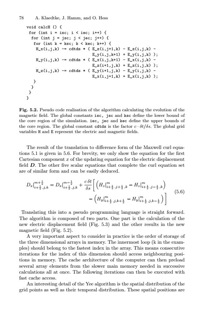
78 A.Klaedtke,J.Hamm,and O.Hess void calcH () for (int i =isc;i iec;i++){ for (int j=jsc;j<jec;j++){ for (int k ksc;k kec;k++){ H_x(i,j,k)-=cdtds *E_z(i,j+1,k)-E_z(i,j,k)- E_y(1,j,k+1)+E-y(i,j,k)); H_y(i,j,k)-=cdtds *E_x(i,j,k+1)-E_x(i,j,k)- E_z(1+1,j,k)+E_z(i,j,k)); H_z(i,j,k)-=cdtds *E_y(i+1,j,k)-E_y(i,j,k)- E_x(i,j+1,k)+E_x(1,j,k)); Fig.5.2.Pseudo code realisation of the algorithm calculating the evolution of the magnetic field.The global constants isc,jsc and ksc define the lower bound of the core region of the simulation.iec,jec and kec define the upper bounds of the core region.The global constant cdtds is the factor c.6t/6s.The global grid variables H and E represent the electric and magnetic fields. The result of the translation to difference form of the Maxwell curl equa- tions 5.1 is given in 5.6.For brevity,we only show the equation for the first Cartesian component r of the updating equation for the electric displacement field D.The other five scalar equations that complete the curl equation set are of similar form and can be easily deduced. cot D==D+[ H册专计5k-H:肝-k (5.6) -(,册5+传-，mk-） Translating this into a pseudo programming language is straight forward. The algorithm is composed of two parts.One part is the calculation of the new electric displacement field (Fig.5.3)and the other results in the new magnetic field (Fig.5.2). A very important aspect to consider in practice is the order of storage of the three dimensional arrays in memory.The innermost loop(k in the exam- ples)should belong to the fastest index in the array.This means consecutive iterations for the index of this dimension should access neighbouring posi- tions in memory.The cache architecture of the computer can then preload several array elements from the slower main memory needed in successive calculations all at once.The following iterations can then be executed with fast cache access. An interesting detail of the Yee algorithm is the spatial distribution of the grid points as well as their temporal distribution.These spatial positions are78 A. Klaedtke, J. Hamm, and O. Hess void calcH () { for (int i = isc; i < iec; i++) { for (int j = jsc; j < jec; j++) { for (int k = ksc; k < kec; k++) { H_x(i,j,k) -= cdtds * ( E_z(i,j+1,k) - E_z(i,j,k) - E_y(i,j,k+1) + E_y(i,j,k) ); H_y(i,j,k) -= cdtds * ( E_x(i,j,k+1) - E_x(i,j,k) - E_z(i+1,j,k) + E_z(i,j,k) ); H_z(i,j,k) -= cdtds * ( E_y(i+1,j,k) - E_y(i,j,k) - E_x(i,j+1,k) + E_x(i,j,k) ); } } } } Fig. 5.2. Pseudo code realisation of the algorithm calculating the evolution of the magnetic field. The global constants isc, jsc and ksc define the lower bound of the core region of the simulation. iec, jec and kec define the upper bounds of the core region. The global constant cdtds is the factor c · δt/δs. The global grid variables H and E represent the electric and magnetic fields. The result of the translation to difference form of the Maxwell curl equa￾tions 5.1 is given in 5.6. For brevity, we only show the equation for the first Cartesian component x of the updating equation for the electric displacement field D. The other five scalar equations that complete the curl equation set are of similar form and can be easily deduced. Dx| m+ 1 2 i+ 1 2 ,j,k = Dx| m− 1 2 i+ 1 2 ,j,k + c δt δs   Hz| m i+ 1 2 ,j+ 1 2 ,k − Hz| m i+ 1 2 ,j− 1 2 ,k −  Hy| m i+ 1 2 ,j,k+ 1 2 − Hy| m i+ 1 2 ,j,k− 1 2   (5.6) Translating this into a pseudo programming language is straight forward. The algorithm is composed of two parts. One part is the calculation of the new electric displacement field (Fig. 5.3) and the other results in the new magnetic field (Fig. 5.2). A very important aspect to consider in practice is the order of storage of the three dimensional arrays in memory. The innermost loop (k in the exam￾ples) should belong to the fastest index in the array. This means consecutive iterations for the index of this dimension should access neighbouring posi￾tions in memory. The cache architecture of the computer can then preload several array elements from the slower main memory needed in successive calculations all at once. The following iterations can then be executed with fast cache access. An interesting detail of the Yee algorithm is the spatial distribution of the grid points as well as their temporal distribution. These spatial positions are