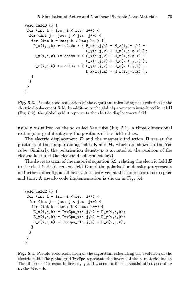
5 Simulation of Active and Nonlinear Photonic Nano-Materials 79 void calcD () for (int i =isc;i iec;i++){ for (int j=jsc;j<jec;j++) for (int k ksc;k kec;k++){ D_x(i,j,k)+=cdtds H_z(i,j,k)-H_z(i,j-1,k)- H_y(1,j,k)+Hy(i,j,k-1)); D_y(i,j,k)+=cdtds (H_x(i,j,k)-H_x(i,j,k-1)- Hz(i,j,k)+Hz(1-1,j,k)); D_z(i,j,k)+=cdtds H_y(i,j,k)-H_y(i-1,j,k)- H_x(1,j,k)+Hx(i,j-1,k)） Fig.5.3.Pseudo code realisation of the algorithm calculating the evolution of the electric displacement field.In addition to the global parameters introduced in calcH (Fig.5.2),the global grid D represents the electric displacement field. usually visualized on the so called Yee cube (Fig.5.1),a three dimensional rectangular grid displaying the positions of the field values. The electric displacement D and the magnetic induction B are at the positions of their appertaining fields E and H,which are shown in the Yee cube.Similarly,the polarisation density p is situated at the position of the electric field and the electric displacement field. The discretisation of the material equation 5.2,relating the electric field E to the electric displacement field D and the polarisation density p represents no further difficulty,as all field values are given at the same positions in space and time.A pseudo code implementation is shown in Fig.5.4. void calcE () for (int i=isc;i<iec;it+){ for (int j=jsc;j<jec;j++){ for (int k ksc;k kec;k++){ E_x(i,j,k)=InvEps_x(i,j,k)D_x(i,j,k) E_y(i,j,k)=InvEps_y(i,j,k)*D_y(i,j,k); E_z(i,j,k)=InvEps_z(i,j,k)*D_z(i,j,k); Fig.5.4.Pseudo code realisation of the algorithm calculating the evolution of the electric field.The global grid InvEps represents the inverse of the er material index. The different Cartesian indices x,y and z account for the spatial offset according to the Yee-cube.5 Simulation of Active and Nonlinear Photonic Nano-Materials 79 void calcD () { for (int i = isc; i < iec; i++) { for (int j = jsc; j < jec; j++) { for (int k = ksc; k < kec; k++) { D_x(i,j,k) += cdtds * ( H_z(i,j,k) - H_z(i,j-1,k) - H_y(i,j,k) + H_y(i,j,k-1) ); D_y(i,j,k) += cdtds * ( H_x(i,j,k) - H_x(i,j,k-1) - H_z(i,j,k) + H_z(i-1,j,k) ); D_z(i,j,k) += cdtds * ( H_y(i,j,k) - H_y(i-1,j,k) - H_x(i,j,k) + H_x(i,j-1,k) ); } } } } Fig. 5.3. Pseudo code realisation of the algorithm calculating the evolution of the electric displacement field. In addition to the global parameters introduced in calcH (Fig. 5.2), the global grid D represents the electric displacement field. usually visualized on the so called Yee cube (Fig. 5.1), a three dimensional rectangular grid displaying the positions of the field values. The electric displacement D and the magnetic induction B are at the positions of their appertaining fields E and H, which are shown in the Yee cube. Similarly, the polarisation density p is situated at the position of the electric field and the electric displacement field. The discretisation of the material equation 5.2, relating the electric field E to the electric displacement field D and the polarisation density p represents no further difficulty, as all field values are given at the same positions in space and time. A pseudo code implementation is shown in Fig. 5.4. void calcE () { for (int i = isc; i < iec; i++) { for (int j = jsc; j < jec; j++) { for (int k = ksc; k < kec; k++) { E_x(i,j,k) = InvEps_x(i,j,k) * D_x(i,j,k); E_y(i,j,k) = InvEps_y(i,j,k) * D_y(i,j,k); E_z(i,j,k) = InvEps_z(i,j,k) * D_z(i,j,k); } } } } Fig. 5.4. Pseudo code realisation of the algorithm calculating the evolution of the electric field. The global grid InvEps represents the inverse of the r material index. The different Cartesian indices x, y and z account for the spatial offset according to the Yee-cube