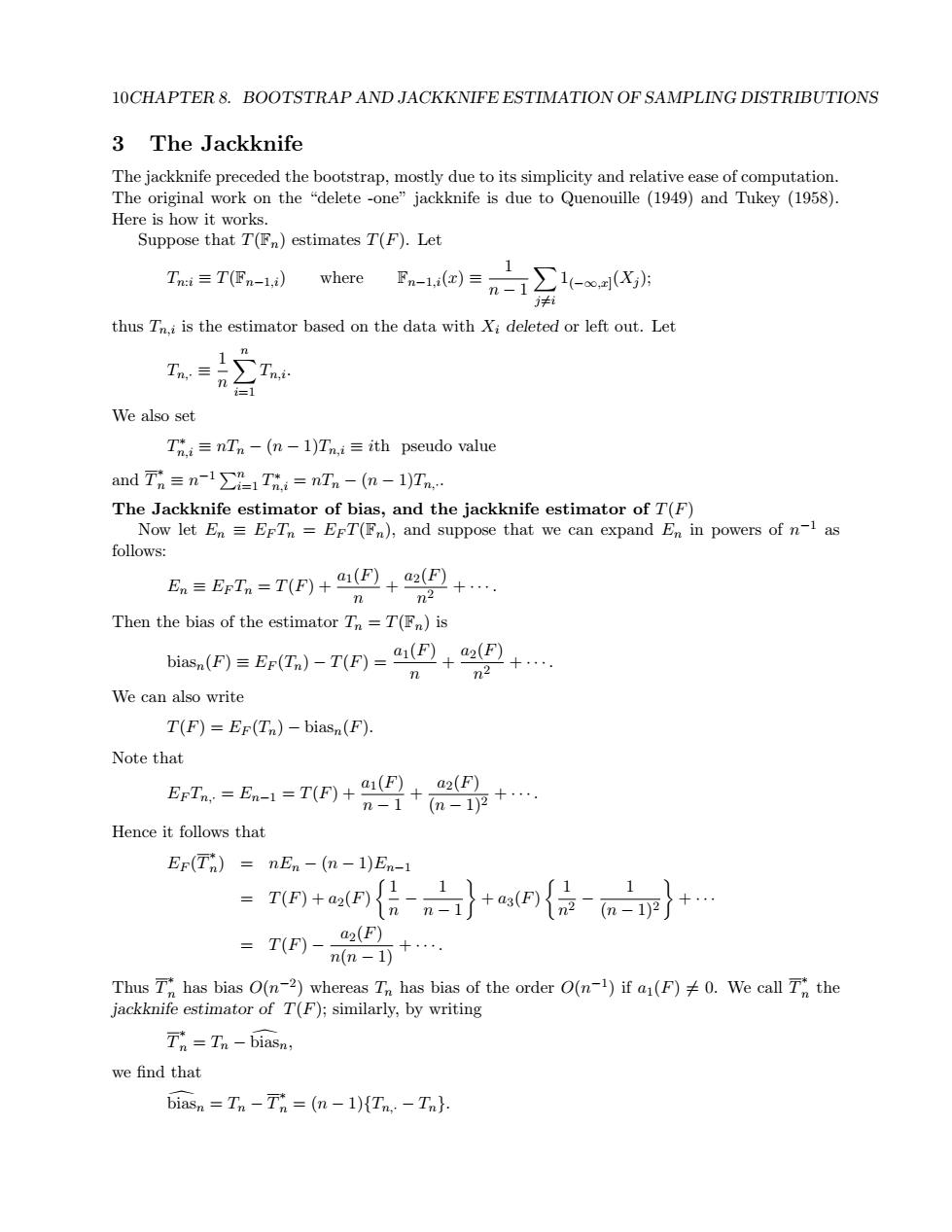
10CHAPTER 8.BOOTSTRAP AND JACKKNIFE ESTIMATION OF SAMPLING DISTRIBUTIONS 3 The Jackknife The jackknife preceded the bootstrap,mostly due to its simplicity and relative ease of computation. The original work on the "delete -one"jackknife is due to Quenouille (1949)and Tukey (1958). Here is how it works. Suppose that T(Fn)estimates T(F).Let Tn:i三T(Fn-l,i) where -1=n-∑-X方 thus Tn.i is the estimator based on the data with Xi deleted or left out.Let n We also set Tta≡nTn-(n-l)Tn,i≡ith pseudo value and Tn≡n-1∑=1Tt&=nTn-(m-1)Tn The Jackknife estimator of bias,and the jackknife estimator of T(F) Now let En=EFTn=ErT(Fn),and suppose that we can expand En in powers of n-1 as follows: En=ErTn=T(F)+)+. n2 Then the bias of the estimator Tn=T(Fn)is biasn(P）=Er(T)-TE）=1(+2E+ n n2 We can also write T(F)=EF(Tn)-biasn(F). Note that 江=-1=0+9++ Hence it follows that EF(Tn)=nEn -(n-1)En-1 n+ar}+asn{信-n}+ = =T(F)- a2(F) n(n-1) 十···。 Thus Tr has bias O(n-2)whereas Tn has bias of the order O(n-1)if a(F)0.We call T the jackknife estimator of T(F);similarly,by writing Tn=Tn -biasn, we find that biasn Tn -Tn (n-1){Tn,-Tn}.10CHAPTER 8. BOOTSTRAP AND JACKKNIFE ESTIMATION OF SAMPLING DISTRIBUTIONS 3 The Jackknife The jackknife preceded the bootstrap, mostly due to its simplicity and relative ease of computation. The original work on the “delete -one” jackknife is due to Quenouille (1949) and Tukey (1958). Here is how it works. Suppose that T(Fn) estimates T(F). Let Tn:i ≡ T(Fn−1,i) where Fn−1,i(x) ≡ 1 n − 1 X j6=i 1(−∞,x] (Xj ); thus Tn,i is the estimator based on the data with Xi deleted or left out. Let Tn,· ≡ 1 n Xn i=1 Tn,i. We also set T ∗ n,i ≡ nTn − (n − 1)Tn,i ≡ ith pseudo value and T ∗ n ≡ n −1 Pn i=1 T ∗ n,i = nTn − (n − 1)Tn,· . The Jackknife estimator of bias, and the jackknife estimator of T(F) Now let En ≡ EF Tn = EF T(Fn), and suppose that we can expand En in powers of n −1 as follows: En ≡ EF Tn = T(F) + a1(F) n + a2(F) n2 + · · · . Then the bias of the estimator Tn = T(Fn) is biasn(F) ≡ EF (Tn) − T(F) = a1(F) n + a2(F) n2 + · · · . We can also write T(F) = EF (Tn) − biasn(F). Note that EF Tn,· = En−1 = T(F) + a1(F) n − 1 + a2(F) (n − 1)2 + · · · . Hence it follows that EF (T ∗ n ) = nEn − (n − 1)En−1 = T(F) + a2(F)  1 n − 1 n − 1  + a3(F)  1 n2 − 1 (n − 1)2  + · · · = T(F) − a2(F) n(n − 1) + · · · . Thus T ∗ n has bias O(n −2 ) whereas Tn has bias of the order O(n −1 ) if a1(F) 6= 0. We call T ∗ n the jackknife estimator of T(F); similarly, by writing T ∗ n = Tn − bias dn, we find that bias dn = Tn − T ∗ n = (n − 1){Tn,· − Tn}