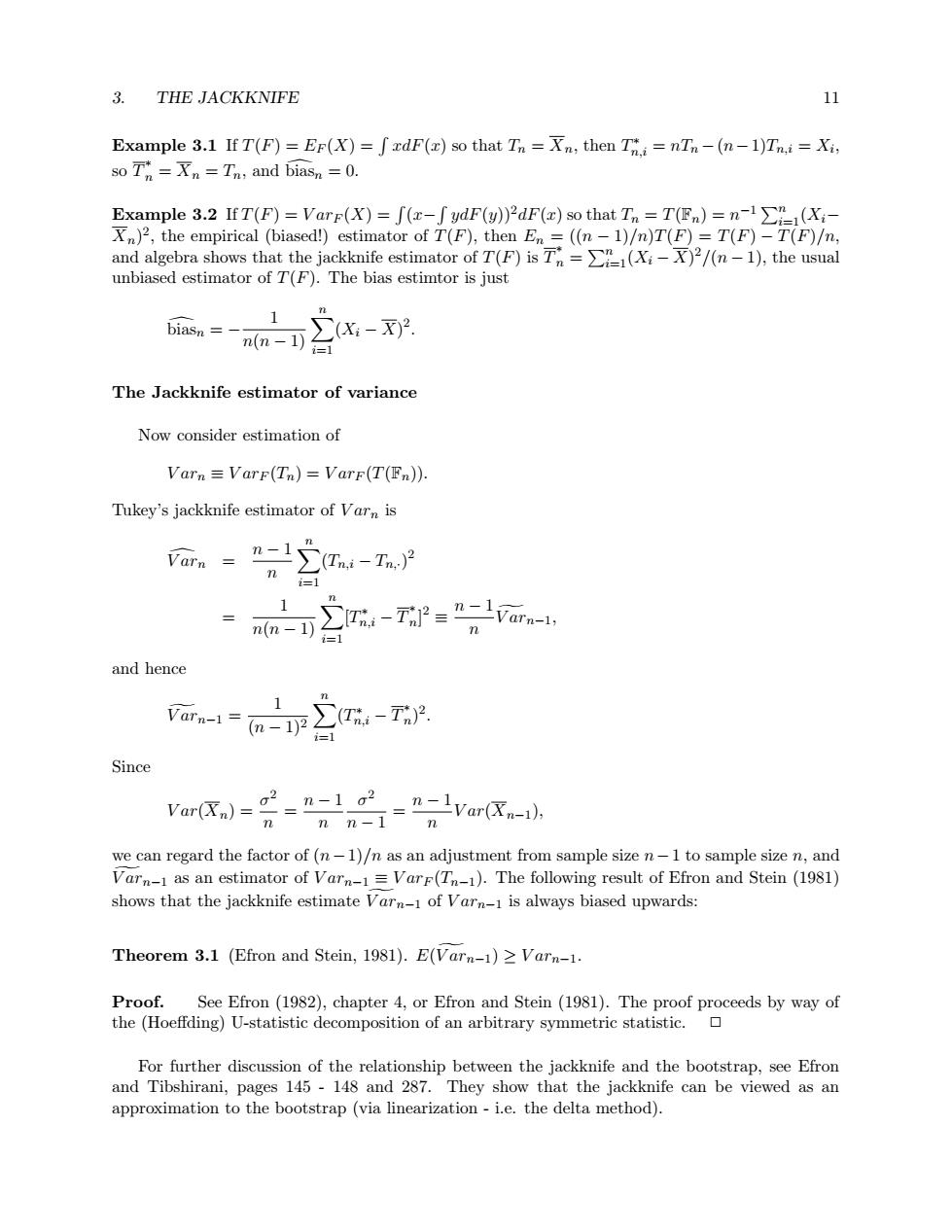
3. THE JACKKNIFE 11 Example 3.1 If T(F)=EF(X)=fxdF(x)so that Tn Xn;then Ti=nTn-(n-1)Tn.i=Xi, so Tr =n =Tn;and biasn =0. Example 3.2 IfT(F)=Varr(X)=f(x-f ydF(y))2dF(z)so that Tn =T(Fn)=n-1>(Xi- Xn)2,the empirical (biased!)estimator of T(F),then En =((n-1)/n)T(F)=T(F)-T(F)/n, and algebra shows that the jackknife estimator of T(F)is T=(Xi-X)2/(n-1),the usual unbiased estimator of T(F).The bias estimtor is just 1 ∑X:-2 n(n-1) The Jackknife estimator of variance Now consider estimation of Varn VarF(Tn)=VarF(T(Fn)). Tukey's jackknife estimator of Varn is a="1∑4- n i=1 1 n(n-1) ∑i-T2=”a-, = and hence 1 ar-1=n-p∑Ta-TP i=1 Since var=g=n=1=n-var风-i n n-I n we can regard the factor of(n-1)/n as an adjustment from sample size n-1 to sample size n,and Varn-1 as an estimator of Varn-1=VarF(Tn-1).The following result of Efron and Stein (1981) shows that the jackknife estimate Varn-1 of Varn-1 is always biased upwards: Theorem 3.1 (Efron and Stein,1981).E(Varn-1)>Varn-1. Proof.See Efron(1982),chapter 4,or Efron and Stein (1981).The proof proceeds by way of the (Hoeffding)U-statistic decomposition of an arbitrary symmetric statistic. For further discussion of the relationship between the jackknife and the bootstrap,see Efron and Tibshirani,pages 145-148 and 287.They show that the jackknife can be viewed as an approximation to the bootstrap (via linearization-i.e.the delta method).3. THE JACKKNIFE 11 Example 3.1 If T(F) = EF (X) = R xdF(x) so that Tn = Xn, then T ∗ n,i = nTn −(n−1)Tn,i = Xi , so T ∗ n = Xn = Tn, and bias dn = 0. Example 3.2 If T(F) = V arF (X) = R (x− R ydF(y))2dF(x) so that Tn = T(Fn) = n −1 Pn i=1(Xi− Xn) 2 , the empirical (biased!) estimator of T(F), then En = ((n − 1)/n)T(F) = T(F) − T(F)/n, and algebra shows that the jackknife estimator of T(F) is T ∗ n = Pn i=1(Xi − X) 2/(n − 1), the usual unbiased estimator of T(F). The bias estimtor is just bias dn = − 1 n(n − 1) Xn i=1 (Xi − X) 2 . The Jackknife estimator of variance Now consider estimation of V arn ≡ V arF (Tn) = V arF (T(Fn)). Tukey’s jackknife estimator of V arn is V ar dn = n − 1 n Xn i=1 (Tn,i − Tn,·) 2 = 1 n(n − 1) Xn i=1 [T ∗ n,i − T ∗ n ] 2 ≡ n − 1 n V ar gn−1, and hence V ar gn−1 = 1 (n − 1)2 Xn i=1 (T ∗ n,i − T ∗ n ) 2 . Since V ar(Xn) = σ 2 n = n − 1 n σ 2 n − 1 = n − 1 n V ar(Xn−1), we can regard the factor of (n−1)/n as an adjustment from sample size n−1 to sample size n, and V ar gn−1 as an estimator of V arn−1 ≡ V arF (Tn−1). The following result of Efron and Stein (1981) shows that the jackknife estimate V ar gn−1 of V arn−1 is always biased upwards: Theorem 3.1 (Efron and Stein, 1981). E(V ar gn−1) ≥ V arn−1. Proof. See Efron (1982), chapter 4, or Efron and Stein (1981). The proof proceeds by way of the (Hoeffding) U-statistic decomposition of an arbitrary symmetric statistic. ✷ For further discussion of the relationship between the jackknife and the bootstrap, see Efron and Tibshirani, pages 145 - 148 and 287. They show that the jackknife can be viewed as an approximation to the bootstrap (via linearization - i.e. the delta method)