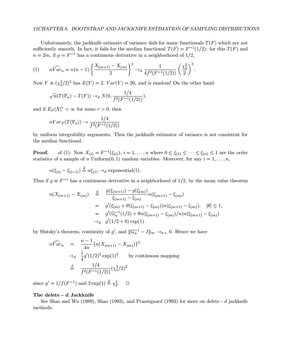
12CHAPTER 8.BOOTSTRAP AND JACKKNIFE ESTIMATION OF SAMPLING DISTRIBUTIONS Unfortunately,the jackknife estimate of variance fails for many functionals T(F)which are not sufficiently smooth.In fact,it fails for the median functional T(F)=F-1(1/2):for this T(F)and n =2m,if g=F-1 has a continuous derivative in a neighborhood of 1/2, (1) nVarn n(n-I ) 2 2 Now Y=(x2/2)2 has E(Y)=2,Var(Y)=20,and is random!On the other hand Vn(T(图)-T(F)→aN0,PE-0/2” 1/4 and if ErX<oo for some r>0,then 1/4 nVarF(T(E》→fF-/2 by uniform integrability arguments.Thus the jackknife estimator of variance is not consistent for the median functional. Proof..of(1):NowX()=F-1(ξg),i=l,.,n where0≤sa)≤…≤sm)≤1 are the order statistics of a sample of n Uniform(0,1)random variables.Moreover,for any i=1,...,n, n(间-fi-l）兰nsu→dexponential(1). Thus if g =F-1 has a continuous derivative in a neighborhood of 1/2,by the mean value theorem n(Xmt)-Xam）±)-(5(mn(m+l-im） ξ(m+1)-5(m) =g(m)+6(ξm+1)）-m)》n(m+1)-5m)）,l9l≤1， =g(Gn1(1/2)+fn(5m+1)-m)/m)n(5m+1)-5m） →ag'(1/2+0)exp(1) by Slutsky's theorem,continuity of g,and G-.0.Hence we have nVarn (n(X(m)m 49(1/2)2exp(1)2 by continuous mapping 1/4 fPF-1/2の/2)2 since g'=1/f(F-1)and 2 exp(1)x. The delete-d Jackknife See Shao and Wu (1989),Shao (1993),and Praestgaard (1993)for more on delete-d jackknife methods.12CHAPTER 8. BOOTSTRAP AND JACKKNIFE ESTIMATION OF SAMPLING DISTRIBUTIONS Unfortunately, the jackknife estimate of variance fails for many functionals T(F) which are not sufficiently smooth. In fact, it fails for the median functional T(F) = F −1 (1/2): for this T(F) and n = 2m, if g = F −1 has a continuous derivative in a neighborhood of 1/2, nV ar dn = n(n − 1)  X(m+1) − X(m) 2 2 →d 1 4f 2(F −1(1/2))  χ 2 2 2 2 (1) . Now Y ≡ (χ 2 2 /2)2 has E(Y ) = 2, V ar(Y ) = 20, and is random! On the other hand √ n(T(Fn) − T(F)) →d N(0, 1/4 f 2(F −1(1/2))), and if EF |X| r < ∞ for some r > 0, then nV arF (T(Fn)) → 1/4 f 2(F −1(1/2)) by uniform integrability arguments. Thus the jackknife estimator of variance is not consistent for the median functional. Proof. of (1): Now X(i) = F −1 (ξ(i) ), i = 1, . . . , n where 0 ≤ ξ(1) ≤ · · · ≤ ξ(n) ≤ 1 are the order statistics of a sample of n Uniform(0, 1) random variables. Moreover, for any i = 1, . . . , n, n(ξ(i) − ξ(i−1)) d= nξ(1) →d exponential(1). Thus if g ≡ F −1 has a continuous derivative in a neighborhood of 1/2, by the mean value theorem n(X(m+1) − X(m) ) d= g(ξ(m+1)) − g(ξ(m) ) ξ(m+1) − ξ(m) n(ξ(m+1) − ξ(m) ) = g 0 (ξ(m) + θ(ξ(m+1) − ξ(m) ))n(ξ(m+1) − ξ(m) ), |θ| ≤ 1, = g 0 (G −1 n (1/2) + θn(ξ(m+1) − ξ(m) )/n)n(ξ(m+1) − ξ(m) ) →d g 0 (1/2 + 0) exp(1) by Slutsky’s theorem, continuity of g 0 , and kG−1 n − Ik∞ →a.s. 0. Hence we have nV ar dn = n − 1 4n {n(X(m+1) − X(m) )} 2 →d 1 4 g 0 (1/2)2 exp(1)2 by continuous mapping d= 1/4 f 2(F −1(1/2))(χ 2 1/2)2 since g 0 = 1/f(F −1 ) and 2 exp(1) d= χ 2 2 . ✷ The delete - d Jackknife See Shao and Wu (1989), Shao (1993), and Praestgaard (1993) for more on delete - d jackknife methods