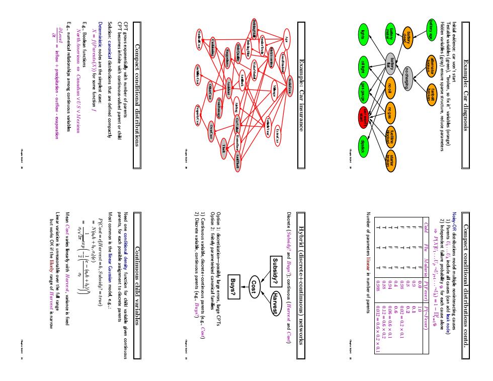
Eumerical relationshipmontinousvariable Compact conditional distributions Example:Car insurance Example:Car diagnosis Continuous child variables Buys? Subsidy?Harvest Discrete [?and Buts?):continuous [Harrest and Cosf) Hybrid (discrete+continuous)networks linear in number of par -02X0 Compact conditional distributions contd. Example: Car diagnosis Initial evidence: car won’t start Testable variables (green), “broken, so fix it” variables (orange) Hidden variables (gray) ensure sparse structure, reduce parameters lights no oil no gas broken starter battery age broken alternator broken fanbelt dead battery no charging flat battery gas gauge blocked fuel line oil light meter battery start car won’t dipstick Chapter 14.1–3 19 Example: Car insurance SocioEcon Age GoodStudent ExtraCar Mileage VehicleYear RiskAversion SeniorTrain DrivingSkill MakeModel DrivingHist DrivQuality Antilock Airbag CarValue HomeBase AntiTheft Theft OwnDamage PropertyCost LiabilityCost MedicalCost Cushioning Ruggedness Accident OtherCost OwnCost Chapter 14.1–3 20 Compact conditional distributions CPT grows exponentially with number of parents CPT becomes infinite with continuous-valued parent or child Solution: canonical distributions that are defined compactly Deterministic nodes are the simplest case: X = f(Parents(X)) for some function f E.g., Boolean functions NorthAmerican ⇔ Canadian ∨ US ∨ Mexican E.g., numerical relationships among continuous variables ∂Level ∂t = inflow + precipitation - outflow - evaporation Chapter 14.1–3 21 Compact conditional distributions contd. Noisy-OR distributions model multiple noninteracting causes 1) Parents U1 . . .Uk include all causes (can add leak node) 2) Independent failure probability qi for each cause alone ⇒ P(X|U1 . . .Uj , ¬Uj+1 . . . ¬Uk) = 1 − Πi j = 1 qi Cold Flu Malaria P(Fever) P(¬Fever) F F F 0.0 1.0 F F T 0.9 0.1 F T F 0.8 0.2 F T T 0.98 0.02 = 0.2 × 0.1 T F F 0.4 0.6 T F T 0.94 0.06 = 0.6 × 0.1 T T F 0.88 0.12 = 0.6 × 0.2 T T T 0.988 0.012 = 0.6 × 0.2 × 0.1 Number of parameters linear in number of parents Chapter 14.1–3 22 Hybrid (discrete+continuous) networks Discrete (Subsidy? and Buys?); continuous (Harvest and Cost) Buys? Harvest Subsidy? Cost Option 1: discretization—possibly large errors, large CPTs Option 2: finitely parameterized canonical families 1) Continuous variable, discrete+continuous parents (e.g., Cost) 2) Discrete variable, continuous parents (e.g., Buys?) Chapter 14.1–3 23 Continuous child variables Need one conditional density function for child variable given continuous parents, for each possible assignment to discrete parents Most common is the linear Gaussian model, e.g.,: P(Cost = c|Harvest = h, Subsidy? = true) = N(ath + bt , σt)(c) = 1 σt √ 2π exp      − 2 1     c − (ath + bt) σt    2      Mean Cost varies linearly with Harvest, variance is fixed Linear variation is unreasonable over the full range but works OK if the likely range of Harvest is narrow Chapter 14.1–3 24