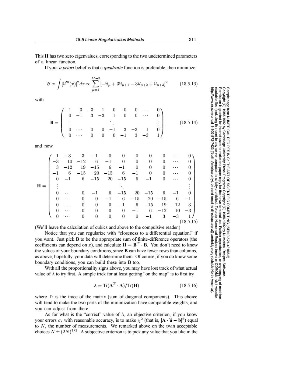
18.5 Linear Regularization Methods 811 This H has two zero eigenvalues,corresponding to the two undetermined parameters of a linear function. If your a priori belief is that a quadratic function is preferable,then minimize M-3 B x "(r)P2dr 立+3u+1-3u+2+i4+3]2 (18.5.13) with -1 3-31 0 0 0… 0 -1 3-3 1 0 0 0 83 B= : (18.5.14) 鱼 0 0 0 -1 3 -3 1 0 0 0 0 -1 3 -3 1 务9 1872 and now 1 -3 3 -1 0 0 0 0 0 0 10-12 6 -1 0 0 0 0 3 -12 19 -15 6 -1 0 0 0 (North America to any server computer, users to make one paper UnN电.t 9 THE -1 6 -15 20 -15 6 -1 0 0 0 ART 0 -1 6 -15 20 -15 6 -1 0 0 H= strictly prohibited Programs 0 E ..E 0 -1 6 -15 20 -15 6 -1 0 send 0 0 -1 6 -15 20 -15 6 -1 0 0 0 0 -1 6 -15 19 -12 0 0 0 0 -1 6 -12 10 3 to dir 0 0 0 0 0 -1 3 -3 1/ (18.5.15) (We'll leave the calculation of cubics and above to the compulsive reader.) OF SCIENTIFIC COMPUTING(ISBN 0-521- Notice that you can regularize with "closeness to a differential equation,"if you want.Just pick B to be the appropriate sum of finite-difference operators(the coefficients can depend on x),and calculate H=BT.B.You don't need to know the values of your boundary conditions,since B can have fewer rows than columns, 1988-1992 by Numerical Recipes as above;hopefully,your data will determine them.Of course,if you do know some -43198.5 boundary conditions,you can build these into B too. (outside With all the proportionality signs above,you may have lost track of what actual value of A to try first.A simple trick for at least getting"on the map"is to first try North Software. 入=Tr(AT·A)/Tr(H) (18.5.16 visit website where Tr is the trace of the matrix(sum of diagonal components).This choice will tend to make the two parts of the minimization have comparable weights,and you can adjust from there. As for what is the "correct value of A,an objective criterion,if you know your errors oi with reasonable accuracy,is to make x2(that is,A.u-b2)equal to N,the number of measurements.We remarked above on the twin acceptable choices N(2N)1/2.A subjective criterion is to pick any value that you like in the18.5 Linear Regularization Methods 811 Permission is granted for internet users to make one paper copy for their own personal use. Further reproduction, or any copyin Copyright (C) 1988-1992 by Cambridge University Press. Programs Copyright (C) 1988-1992 by Numerical Recipes Software. Sample page from NUMERICAL RECIPES IN C: THE ART OF SCIENTIFIC COMPUTING (ISBN 0-521-43108-5) g of machine￾readable files (including this one) to any server computer, is strictly prohibited. To order Numerical Recipes books or CDROMs, visit website http://www.nr.com or call 1-800-872-7423 (North America only), or send email to directcustserv@cambridge.org (outside North America). This H has two zero eigenvalues, corresponding to the two undetermined parameters of a linear function. If your a priori belief is that a quadratic function is preferable, then minimize B ∝
[u


(x)]2dx ∝ M −3 µ=1 [−uµ + 3uµ+1 − 3uµ+2 + uµ+3] 2 (18.5.13) with B =   −1 3 −31000 ··· 0 0 −1 3 −3100 ··· 0 . . . ... . . . 0 ··· 0 0 −1 3 −310 0 ··· 000 −1 3 −3 1   (18.5.14) and now H =   1 −3 3 −100000 ··· 0 −3 10 −12 6 −10000 ··· 0 3 −12 19 −15 6 −1000 ··· 0 −1 6 −15 20 −15 6 −100 ··· 0 0 −1 6 −15 20 −15 6 −1 0 ··· 0 . . . ... . . . 0 ··· 0 −1 6 −15 20 −15 6 −1 0 0 ··· 0 0 −1 6 −15 20 −15 6 −1 0 ··· 000 −1 6 −15 19 −12 3 0 ··· 0000 −1 6 −12 10 −3 0 ··· 00000 −1 3 −3 1   (18.5.15) (We’ll leave the calculation of cubics and above to the compulsive reader.) Notice that you can regularize with “closeness to a differential equation,” if you want. Just pick B to be the appropriate sum of finite-difference operators (the coefficients can depend on x), and calculate H = BT · B. You don’t need to know the values of your boundary conditions, since B can have fewer rows than columns, as above; hopefully, your data will determine them. Of course, if you do know some boundary conditions, you can build these into B too. With all the proportionality signs above, you may have lost track of what actual value of λ to try first. A simple trick for at least getting “on the map” is to first try λ = Tr(AT · A)/Tr(H) (18.5.16) where Tr is the trace of the matrix (sum of diagonal components). This choice will tend to make the two parts of the minimization have comparable weights, and you can adjust from there. As for what is the “correct” value of λ, an objective criterion, if you know your errors σi with reasonable accuracy, is to make χ2 (that is, |A · u − b| 2) equal to N, the number of measurements. We remarked above on the twin acceptable choices N ± (2N)1/2. A subjective criterion is to pick any value that you like in the