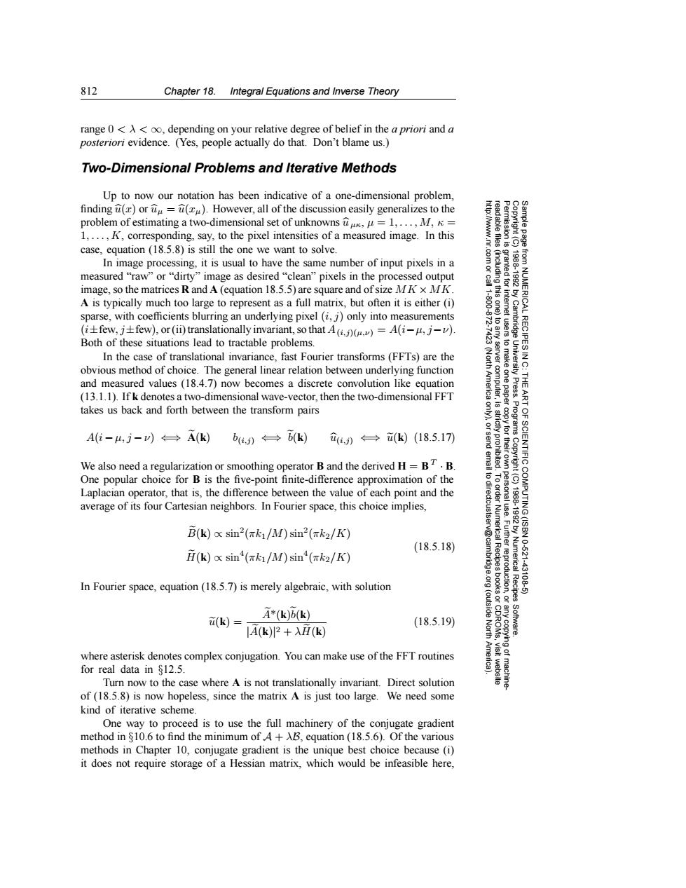
812 Chapter 18.Integral Equations and Inverse Theory range 0<A<oo,depending on your relative degree of belief in the a priori and a posteriori evidence.(Yes,people actually do that.Don't blame us.) Two-Dimensional Problems and Iterative Methods Up to now our notation has been indicative of a one-dimensional problem, finding ()or=().However,all of the discussion easily generalizes to the problem of estimating a two-dimensional set of unknowns=1,...,M,K= 1,...,K,corresponding,say,to the pixel intensities of a measured image.In this case,equation(18.5.8)is still the one we want to solve. 三 81 In image processing,it is usual to have the same number of input pixels in a measured“raw'or“dirty'image as desired“clean”pixels in the processed output image,so the matrices R and A(equation 18.5.5)are square and of size MK x MK. A is typically much too large to represent as a full matrix,but often it is either(i) sparse,with coefficients blurring an underlying pixel(i,j)only into measurements (ifew,j+few),or(ii)translationally invariant,so that A(i)()=A(i-u,j-v). Both of these situations lead to tractable problems. RECIPES In the case of translational invariance,fast Fourier transforms(FFTs)are the obvious method of choice.The general linear relation between underlying function 9 and measured values(18.4.7)now becomes a discrete convolution like equation (13.1.1).Ifk denotes a two-dimensional wave-vector.then the two-dimensional FFT takes us back and forth between the transform pairs A(i-4,j-w)）←→A(k)ba)←→b(k) ,)←→i(k)(18.5.17) S3 We also need a regularization or smoothing operator B and the derived H=BT.B. One popular choice for B is the five-point finite-difference approximation of the 6 Laplacian operator,that is,the difference between the value of each point and the average of its four Cartesian neighbors.In Fourier space,this choice implies, B(k)xsin2(πk1/M)sin2(πk2/K) (18.5.18) H(k)o sin(1/M)sin(k2/K) Numerica 10621 43126 In Fourier space,equation(18.5.7)is merely algebraic,with solution A*(k)b(k) u(k)= (18.5.19) |A(k)P+入H(k) North where asterisk denotes complex conjugation.You can make use of the FFT routines for real data in 812.5 Turn now to the case where A is not translationally invariant.Direct solution of(18.5.8)is now hopeless,since the matrix A is just too large.We need some kind of iterative scheme. One way to proceed is to use the full machinery of the conjugate gradient method in 810.6 to find the minimum ofA+AB,equation (18.5.6).Of the various methods in Chapter 10,conjugate gradient is the unique best choice because (1) it does not require storage of a Hessian matrix,which would be infeasible here,812 Chapter 18. Integral Equations and Inverse Theory Permission is granted for internet users to make one paper copy for their own personal use. Further reproduction, or any copyin Copyright (C) 1988-1992 by Cambridge University Press. Programs Copyright (C) 1988-1992 by Numerical Recipes Software. Sample page from NUMERICAL RECIPES IN C: THE ART OF SCIENTIFIC COMPUTING (ISBN 0-521-43108-5) g of machine￾readable files (including this one) to any server computer, is strictly prohibited. To order Numerical Recipes books or CDROMs, visit website http://www.nr.com or call 1-800-872-7423 (North America only), or send email to directcustserv@cambridge.org (outside North America). range 0 <λ< ∞, depending on your relative degree of belief in the a priori and a posteriori evidence. (Yes, people actually do that. Don’t blame us.) Two-Dimensional Problems and Iterative Methods Up to now our notation has been indicative of a one-dimensional problem, finding u(x) or uµ = u(xµ). However, all of the discussion easily generalizes to the problem of estimating a two-dimensional set of unknowns uµκ, µ = 1,...,M, κ = 1,...,K, corresponding, say, to the pixel intensities of a measured image. In this case, equation (18.5.8) is still the one we want to solve. In image processing, it is usual to have the same number of input pixels in a measured “raw” or “dirty” image as desired “clean” pixels in the processed output image, so the matrices R and A (equation 18.5.5) are square and of size MK ×MK. A is typically much too large to represent as a full matrix, but often it is either (i) sparse, with coefficients blurring an underlying pixel (i, j) only into measurements (i±few, j±few), or (ii) translationally invariant, so that A(i,j)(µ,ν) = A(i−µ, j−ν). Both of these situations lead to tractable problems. In the case of translational invariance, fast Fourier transforms (FFTs) are the obvious method of choice. The general linear relation between underlying function and measured values (18.4.7) now becomes a discrete convolution like equation (13.1.1). If k denotes a two-dimensional wave-vector, then the two-dimensional FFT takes us back and forth between the transform pairs A(i − µ, j − ν) ⇐⇒ A(k) b(i,j) ⇐⇒ b(k) u(i,j) ⇐⇒ u(k) (18.5.17) We also need a regularization or smoothing operator B and the derived H = B T · B. One popular choice for B is the five-point finite-difference approximation of the Laplacian operator, that is, the difference between the value of each point and the average of its four Cartesian neighbors. In Fourier space, this choice implies, B(k) ∝ sin2(πk1/M) sin2(πk2/K) H(k) ∝ sin4(πk1/M) sin4(πk2/K) (18.5.18) In Fourier space, equation (18.5.7) is merely algebraic, with solution u(k) = A*(k)b(k) |A(k)| 2 + λH(k) (18.5.19) where asterisk denotes complex conjugation. You can make use of the FFT routines for real data in §12.5. Turn now to the case where A is not translationally invariant. Direct solution of (18.5.8) is now hopeless, since the matrix A is just too large. We need some kind of iterative scheme. One way to proceed is to use the full machinery of the conjugate gradient method in §10.6 to find the minimum of A + λB, equation (18.5.6). Of the various methods in Chapter 10, conjugate gradient is the unique best choice because (i) it does not require storage of a Hessian matrix, which would be infeasible here,