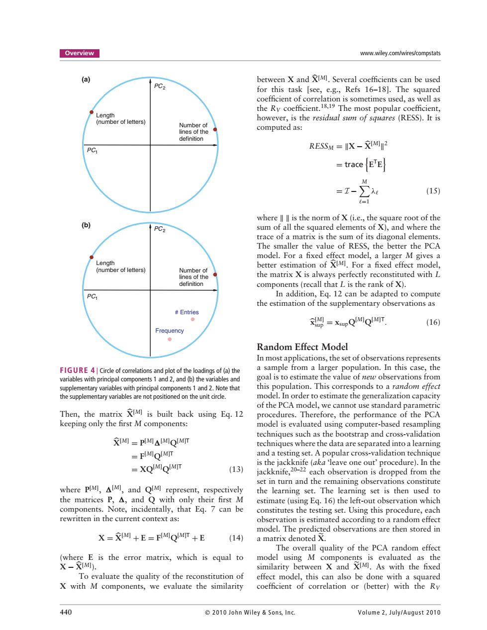
Overview www.wiley.com/wires/compstats (a) between X and XIMI.Several coefficients can be used PC2 for this task [see,e.g.,Refs 16-18].The squared coefficient of correlation is sometimes used,as well as the Ry coefficient.18.19 The most popular coefficient, Length (number of letters) however,is the residual sum of squares (RESS).It is Number of computed as: lines of the definition PC RESSM IX-XIMI2 traceETE =I- ∑ (15) =1 where ll ll is the norm of X(i.e.,the square root of the (b) PC2 sum of all the squared elements of X),and where the trace of a matrix is the sum of its diagonal elements. The smaller the value of RESS,the better the PCA model.For a fixed effect model,a larger M gives a Length better estimation of XIMI.For a fixed effect model, (number of letters) Number of lines of the the matrix X is always perfectly reconstituted with L definition components (recall that L is the rank of X). PC In addition,Eq.12 can be adapted to compute the estimation of the supplementary observations as Entries 单 =xpQIMIQIMIT (16) Frequency ● Random Effect Model In most applications,the set of observations represents FIGURE 4 Circle of correlations and plot of the loadings of (a)the a sample from a larger population.In this case,the variables with principal components 1 and 2,and (b)the variables and goal is to estimate the value of net observations from supplementary variables with principal components 1 and 2.Note that this population.This corresponds to a random effect the supplementary variables are not positioned on the unit circle. model.In order to estimate the generalization capacity of the PCA model,we cannot use standard parametric Then,the matrix XIMI is built back using Eq.12 procedures.Therefore,the performance of the PCA keeping only the first M components: model is evaluated using computer-based resampling techniques such as the bootstrap and cross-validation XIMI PIMIAIMIOIMIT techniques where the data are separated into a learning FIMIOIMIT and a testing set.A popular cross-validation technique =XQIMIOIMIT is the jackknife (aka 'leave one out'procedure).In the (13) jackknife,20-22 each observation is dropped from the set in turn and the remaining observations constitute where PlMI,AIMI,and QIMI represent,respectively the learning set.The learning set is then used to the matrices P,△，and Q with only their first M estimate (using Eq.16)the left-out observation which components.Note,incidentally,that Eq.7 can be constitutes the testing set.Using this procedure,each rewritten in the current context as: observation is estimated according to a random effect model.The predicted observations are then stored in X =XIMI+E=FIMIQIMIT +E (14) a matrix denoted X. The overall quality of the PCA random effect (where E is the error matrix,which is equal to model using M components is evaluated as the X-XIMI). similarity between X and XIMI.As with the fixed To evaluate the quality of the reconstitution of effect model,this can also be done with a squared X with M components,we evaluate the similarity coefficient of correlation or (better)with the Ry 440 2010 John Wiley Sons,Inc. Volume 2,July/August 2010Overview www.wiley.com/wires/compstats PC2 Number of lines of the definition PC1 Length (number of letters) PC2 Number of lines of the definition PC1 Length (number of letters) # Entries Frequency (a) (b) FIGURE 4 | Circle of correlations and plot of the loadings of (a) the variables with principal components 1 and 2, and (b) the variables and supplementary variables with principal components 1 and 2. Note that the supplementary variables are not positioned on the unit circle. Then, the matrix X+[M] is built back using Eq. 12 keeping only the first M components: X+[M] = P[M] ![M] Q[M]T = F[M] Q[M]T = XQ[M] Q[M]T (13) where P[M] , ![M] , and Q[M] represent, respectively the matrices P, !, and Q with only their first M components. Note, incidentally, that Eq. 7 can be rewritten in the current context as: X = X+[M] + E = F[M] Q[M]T + E (14) (where E is the error matrix, which is equal to X − X+[M] ). To evaluate the quality of the reconstitution of X with M components, we evaluate the similarity between X and X+[M] . Several coefficients can be used for this task [see, e.g., Refs 16–18]. The squared coefficient of correlation is sometimes used, as well as the RV coefficient.18,19 The most popular coefficient, however, is the residual sum of squares (RESS). It is computed as: RESSM = &X − X+[M] &2 = trace , ETE - = I −# M #=1 λ# (15) where & & is the norm of X (i.e., the square root of the sum of all the squared elements of X), and where the trace of a matrix is the sum of its diagonal elements. The smaller the value of RESS, the better the PCA model. For a fixed effect model, a larger M gives a better estimation of X+[M] . For a fixed effect model, the matrix X is always perfectly reconstituted with L components (recall that L is the rank of X). In addition, Eq. 12 can be adapted to compute the estimation of the supplementary observations as +x[M] sup = xsupQ[M] Q[M]T. (16) Random Effect Model In most applications, the set of observations represents a sample from a larger population. In this case, the goal is to estimate the value of new observations from this population. This corresponds to a random effect model. In order to estimate the generalization capacity of the PCA model, we cannot use standard parametric procedures. Therefore, the performance of the PCA model is evaluated using computer-based resampling techniques such as the bootstrap and cross-validation techniques where the data are separated into a learning and a testing set. A popular cross-validation technique is the jackknife (aka ‘leave one out’ procedure). In the jackknife,20–22 each observation is dropped from the set in turn and the remaining observations constitute the learning set. The learning set is then used to estimate (using Eq. 16) the left-out observation which constitutes the testing set. Using this procedure, each observation is estimated according to a random effect model. The predicted observations are then stored in a matrix denoted X.. The overall quality of the PCA random effect model using M components is evaluated as the similarity between X and X.[M] . As with the fixed effect model, this can also be done with a squared coefficient of correlation or (better) with the RV 440  2010 John Wiley & Son s, In c. Volume 2, July/Augu st 2010