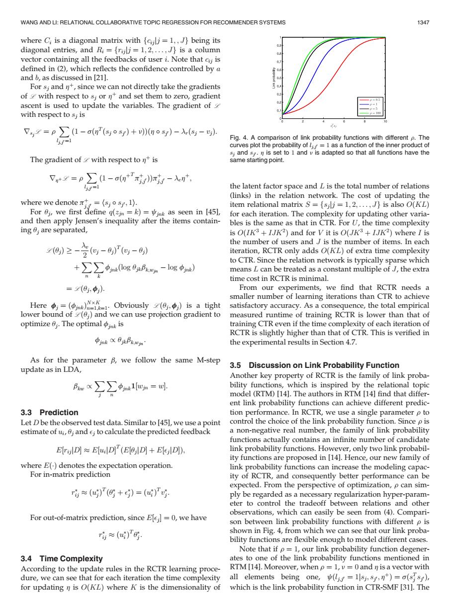
WANG AND LI:RELATIONAL COLLABORATIVE TOPIC REGRESSION FOR RECOMMENDER SYSTEMS 1347 where C;is a diagonal matrix with (ciilj=1,,J}being its diagonal entries,and Ri=[rijlj =1,2,...,J}is a column vector containing all the feedbacks of user i.Note that cij is defined in (2),which reflects the confidence controlled by a 0. and b,as discussed in [21]. For s;and n+,since we can not directly take the gradients 0. of with respect to sj or n and set them to zero,gradient ascent is used to update the variables.The gradient of with respect to sj is 三P之-s°s)+o-- Fig.4.A comparison of link probability functions with different p.The curves plot the probability of l;=1 as a function of the inner product of s;and s,.n is set to 1 and v is adapted so that all functions have the The gradient of with respect to nt is same starting point. 了ty=p∑1-atx》z克-入n, 材=1 the latent factor space and L is the total number of relations (links)in the relation network.The cost of updating the where we denoteπ=(s;os,l） item relational matrix S={sjlj=1,2,....J is also O(KL) For 0j,we first define q(zjn=k)=vink as seen in [451, for each iteration.The complexity for updating other varia- and then apply Jensen's inequality after the items contain- bles is the same as that in CTR.For U,the time complexity ing are separated, is O(IK3+IJK2)and for V it is O(JK3+1JK2)where I is the number of users andJ is the number of items.In each %)≥-合g-Pg- iteration,RCTR only adds O(KL)of extra time complexity +∑∑pog日PE.wm-log9) to CTR.Since the relation network is typically sparse which means L can be treated as a constant multiple of/,the extra 程k time cost in RCTR is minimal. =(0,φ)： From our experiments,we find that RCTR needs a smaller number of learning iterations than CTR to achieve Here中=(ot)k-·Obviously(0,p,）is a tight satisfactory accuracy.As a consequence,the total empirical lower bound of (;and we can use projection gradient to measured runtime of training RCTR is lower than that of optimize 0.The optimal is training CTR even if the time complexity of each iteration of RCTR is slightly higher than that of CTR.This is verified in 中mk0X0ikPk.wn the experimental results in Section 4.7. As for the parameter B,we follow the same M-step update as in LDA, 3.5 Discussion on Link Probability Function Another key property of RCTR is the family of link proba- Bex∑∑mlom=叫 bility functions,which is inspired by the relational topic model(RTM)[14].The authors in RTM [14]find that differ- ent link probability functions can achieve different predic- 3.3 Prediction tion performance.In RCTR,we use a single parameter p to Let D be the observed test data.Similar to [45],we use a point control the choice of the link probability function.Since p is estimate of ui,0;and ej to calculate the predicted feedback a non-negative real number,the family of link probability functions actually contains an infinite number of candidate E(rilD]EluilD](E[ejD]+ElejlD]), link probability functions.However,only two link probabil- ity functions are proposed in [141.Hence,our new family of where E(.)denotes the expectation operation. link probability functions can increase the modeling capac- For in-matrix prediction ity of RCTR,and consequently better performance can be expected.From the perspective of optimization,p can sim- r旁≈(u）)'(+)=(4)' ply be regarded as a necessary regularization hyper-param- eter to control the tradeoff between relations and other observations,which can easily be seen from(4).Compari- For out-of-matrix prediction,since Elej]=0,we have son between link probability functions with different p is 暗≈()' shown in Fig.4,from which we can see that our link proba- bility functions are flexible enough to model different cases. Note that if p=1,our link probability function degener- 3.4 Time Complexity ates to one of the link probability functions mentioned in According to the update rules in the RCTR learning proce- RTM[14].Moreover,when p =1,v=0 and n is a vector with dure,we can see that for each iteration the time complexity all elements being one,(li =1lsj,sy,n+)=a(sfs), for updating n is O(KL)where K is the dimensionality of which is the link probability function in CTR-SMF [31].Thewhere Ci is a diagonal matrix with fcijjj ¼ 1;;Jg being its diagonal entries, and Ri ¼ frijjj ¼ 1; 2; ... ; Jg is a column vector containing all the feedbacks of user i. Note that cij is defined in (2), which reflects the confidence controlled by a and b, as discussed in [21]. For sj and hþ, since we can not directly take the gradients of L with respect to sj or hþ and set them to zero, gradient ascent is used to update the variables. The gradient of L with respect to sj is rsjL ¼ r X l j;j0¼1 ð1 sðhT ðsj  sj0Þ þ nÞÞðh  sj0Þ rðsj vjÞ: The gradient of L with respect to hþ is rhþ L ¼ r X l j;j0¼1 ð1 sðhþT pþ j;j0ÞÞpþ j;j0 ehþ; where we denote pþ j;j0 ¼ hsj  sj0 ; 1i. For uj, we first define qðzjn ¼ kÞ ¼ cjnk as seen in [45], and then apply Jensen’s inequality after the items contain￾ing uj are separated, L ðujÞ v 2 ðvj ujÞ T ðvj ujÞ þX n X k fjnkðlog ujkbk;wjn log fjnkÞ ¼ L ðuj; fjÞ: Here fj ¼ ðfjnkÞ NK n¼1;k¼1. Obviously L ðuj; fjÞ is a tight lower bound of L ðujÞ and we can use projection gradient to optimize uj. The optimal fjnk is fjnk / ujkbk;wjn : As for the parameter b, we follow the same M-step update as in LDA, bkw / X j X n fjnk1½wjn ¼ w : 3.3 Prediction Let D be the observed test data. Similar to [45], we use a point estimate of ui, uj and j to calculate the predicted feedback E½rijjD E½uijD T ðE½ujjD þ E½jjD Þ; where EðÞ denotes the expectation operation. For in-matrix prediction r ij ðu j Þ T ðu j þ  j Þ¼ðu iÞ T v j : For out-of-matrix prediction, since E½j ¼ 0, we have r ij ðu iÞ T u j : 3.4 Time Complexity According to the update rules in the RCTR learning proce￾dure, we can see that for each iteration the time complexity for updating h is OðKLÞ where K is the dimensionality of the latent factor space and L is the total number of relations (links) in the relation network. The cost of updating the item relational matrix S ¼ fsjjj ¼ 1; 2; ... ; Jg is also OðKLÞ for each iteration. The complexity for updating other varia￾bles is the same as that in CTR. For U, the time complexity is OðIK3 þ IJK2Þ and for V it is OðJK3 þ IJK2Þ where I is the number of users and J is the number of items. In each iteration, RCTR only adds OðKLÞ of extra time complexity to CTR. Since the relation network is typically sparse which means L can be treated as a constant multiple of J, the extra time cost in RCTR is minimal. From our experiments, we find that RCTR needs a smaller number of learning iterations than CTR to achieve satisfactory accuracy. As a consequence, the total empirical measured runtime of training RCTR is lower than that of training CTR even if the time complexity of each iteration of RCTR is slightly higher than that of CTR. This is verified in the experimental results in Section 4.7. 3.5 Discussion on Link Probability Function Another key property of RCTR is the family of link proba￾bility functions, which is inspired by the relational topic model (RTM) [14]. The authors in RTM [14] find that differ￾ent link probability functions can achieve different predic￾tion performance. In RCTR, we use a single parameter r to control the choice of the link probability function. Since r is a non-negative real number, the family of link probability functions actually contains an infinite number of candidate link probability functions. However, only two link probabil￾ity functions are proposed in [14]. Hence, our new family of link probability functions can increase the modeling capac￾ity of RCTR, and consequently better performance can be expected. From the perspective of optimization, r can sim￾ply be regarded as a necessary regularization hyper-param￾eter to control the tradeoff between relations and other observations, which can easily be seen from (4). Compari￾son between link probability functions with different r is shown in Fig. 4, from which we can see that our link proba￾bility functions are flexible enough to model different cases. Note that if r ¼ 1, our link probability function degener￾ates to one of the link probability functions mentioned in RTM [14]. Moreover, when r ¼ 1, n ¼ 0 and h is a vector with all elements being one, cðlj;j0 ¼ 1jsj; sj0 ; hþÞ ¼ sðsT j sj0Þ, which is the link probability function in CTR-SMF [31]. The Fig. 4. A comparison of link probability functions with different r. The curves plot the probability of lj;j0 ¼ 1 as a function of the inner product of sj and sj0. h is set to 1 and n is adapted so that all functions have the same starting point. WANG AND LI: RELATIONAL COLLABORATIVE TOPIC REGRESSION FOR RECOMMENDER SYSTEMS 1347