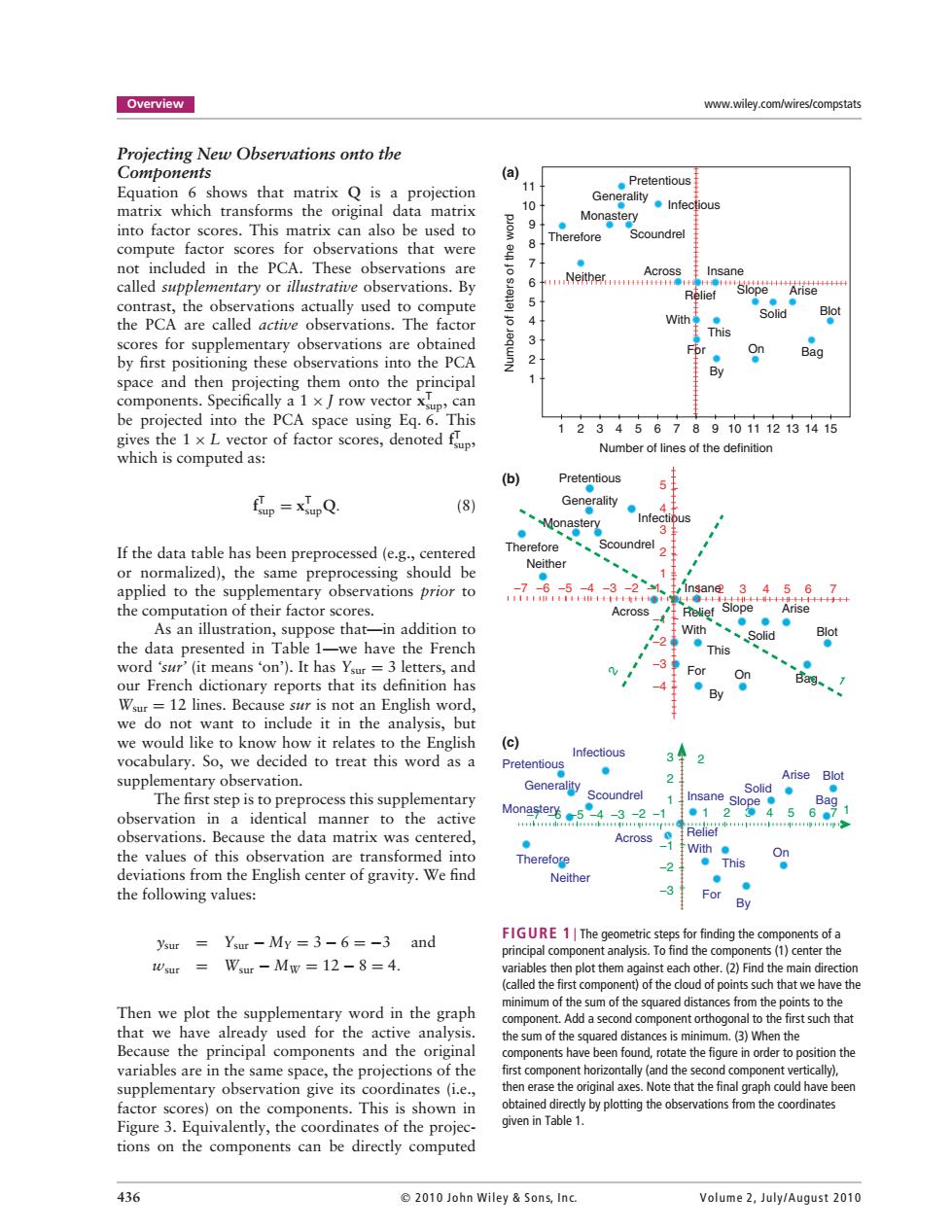
Overview www.wiley.com/wires/compstats Projecting New Observations onto the Components (a) Equation 6 shows that matrix Q is a projection 11 .Pretentious Generality matrix which transforms the original data matrix 10 ●Infectious into factor scores.This matrix can also be used to 9 Monastery ● Therefore Scoundrel compute factor scores for observations that were not included in the PCA.These observations are ● Across Insane called supplementary or illustrative observations.By 6Ne种ea信"5i68Aise Relief contrast,the observations actually used to compute 51 ● 6 With Solid Blot the PCA are called active observations.The factor This scores for supplementary observations are obtained On Bag by first positioning these observations into the PCA ● space and then projecting them onto the principal components.Specifically a 1xJrow vector can be projected into the PCA space using Eq.6.This gives the 1xL vector of factor scores,denoted 123456789101112131415 Number of lines of the definition which is computed as: (b) Pretentious ● 5 fup=xupQ (8) Generality ● 4 Monastery Infectious ● ● 3士 If the data table has been preprocessed (e.g.,centered Therefore 、Scoundrel 2 Neither or normalized),the same preprocessing should be ● 1 applied to the supplementary observations prior to Insane 3 456 7 +十+ the computation of their factor scores. Across As an illustration,suppose that-in addition to With Blot the data presented in Table 1-we have the French 2 Tis ● word 'sur'(it means 'on').It has Ysur =3 letters,and -30 For On our French dictionary reports that its definition has ● Bags Wsur =12 lines.Because sur is not an English word, we do not want to include it in the analysis,but we would like to know how it relates to the English (c) vocabulary.So,we decided to treat this word as a Infectious Pretentious 34 2 ● supplementary observation. Arise Blot Generality Scoundrel Solid● The first step is to preprocess this supplementary 1 Monastery Insane Slope● Bag observation in a identical manner to the active ye%5-434 observations.Because the data matrix was centered, Across With● the values of this observation are transformed into Therefore On -2 ●This ● deviations from the English center of gravity.We find Neither the following values: 3 ●● For By ysur Ysur -My=3-6=-3 and FIGURE 1 The geometric steps for finding the components of a principal component analysis.To find the components (1)center the Wsur Wsur -Mw =12-8=4. variables then plot them against each other.(2)Find the main direction (called the first component)of the cloud of points such that we have the minimum of the sum of the squared distances from the points to the Then we plot the supplementary word in the graph component.Add a second component orthogonal to the first such that that we have already used for the active analysis. the sum of the squared distances is minimum.(3)When the Because the principal components and the original components have been found,rotate the figure in order to position the variables are in the same space,the projections of the first component horizontally (and the second component vertically), supplementary observation give its coordinates (i.e., then erase the original axes.Note that the final graph could have been factor scores)on the components.This is shown in obtained directly by plotting the observations from the coordinates Figure 3.Equivalently,the coordinates of the projec- given in Table 1. tions on the components can be directly computed 436 2010 John Wiley Sons,Inc. Volume 2,July/August 2010Overview www.wiley.com/wires/compstats Projecting New Observations onto the Components Equation 6 shows that matrix Q is a projection matrix which transforms the original data matrix into factor scores. This matrix can also be used to compute factor scores for observations that were not included in the PCA. These observations are called supplementary or illustrative observations. By contrast, the observations actually used to compute the PCA are called active observations. The factor scores for supplementary observations are obtained by first positioning these observations into the PCA space and then projecting them onto the principal components. Specifically a 1 × J row vector xT sup, can be projected into the PCA space using Eq. 6. This gives the 1 × L vector of factor scores, denoted fT sup, which is computed as: f T sup = xT supQ. (8) If the data table has been preprocessed (e.g., centered or normalized), the same preprocessing should be applied to the supplementary observations prior to the computation of their factor scores. As an illustration, suppose that—in addition to the data presented in Table 1—we have the French word ‘sur’ (it means ‘on’). It has Ysur = 3 letters, and our French dictionary reports that its definition has Wsur = 12 lines. Because sur is not an English word, we do not want to include it in the analysis, but we would like to know how it relates to the English vocabulary. So, we decided to treat this word as a supplementary observation. The first step is to preprocess this supplementary observation in a identical manner to the active observations. Because the data matrix was centered, the values of this observation are transformed into deviations from the English center of gravity. We find the following values: ysur = Ysur − MY = 3 − 6 = −3 and wsur = Wsur − MW = 12 − 8 = 4. Then we plot the supplementary word in the graph that we have already used for the active analysis. Because the principal components and the original variables are in the same space, the projections of the supplementary observation give its coordinates (i.e., factor scores) on the components. This is shown in Figure 3. Equivalently, the coordinates of the projec￾tions on the components can be directly computed 9 8 7 6 5 4 3 2 1 2 4 3 5 6 7 9 10 11 12 13 14 15 10 Monastery Number of lines of the definition This For On Bag Solid Blot Across Insane Relief By Arise With Generality Scoundrel Infectious Pretentious Therefore Slope Neither Number of letters of the word 11 1 8 Across Insane Infectious −7 −6 −5 −4 −3 23 456 7 Monastery Pretentious Relief This By For With On Bag Blot Solid Arise Generality Scoundrel 1 2 1 Neither −4 −1 −3 −2 −2 −1 Slope Therefore 1 2 3 4 5 −1 Across Infectious Bag Relief 3 −1 −3 −7 −6 −4 −3 −2 −2 1 2 Monastery Therefore Neither By This Slope Arise Solid With On For Scoundrel Generality Pretentious Blot Insane 2 4 5 6 7 1 1 2 3 (a) (b) (c) −5 FIGURE 1 | The geometric steps for finding the components of a principal component analysis. To find the components (1) center the variables then plot them against each other. (2) Find the main direction (called the first component) of the cloud of points such that we have the minimum of the sum of the squared distances from the points to the component. Add a second component orthogonal to the first such that the sum of the squared distances is minimum. (3) When the components have been found, rotate the figure in order to position the first component horizontally (and the second component vertically), then erase the original axes. Note that the final graph could have been obtained directly by plotting the observations from the coordinates given in Table 1. 436  2010 John Wiley & Son s, In c. Volume 2, July/Augu st 2010