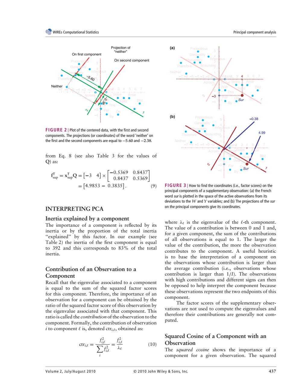
WIREs Computational Statistics Principal component analysis Projection of (a) "neither" On first component On second component 5.60 Neither (b) -0.38 FIGURE 2 Plot of the centered data,with the first and second 499 components.The projections (or coordinates)of the word 'neither'on the first and the second components are equal to-5.60 and-2.38. from Eg.8 (see also Table 3 for the values of Q)as: fp=xpQ=[-34]× -0.53690.8437 0.84370.5369 =[4.9853-0.38351 (9) FIGURE 3|How to find the coordinates (i.e.,factor scores)on the principal components of a supplementary observation:(a)the French word sur is plotted in the space of the active observations from its deviations to the W and Y variables;and (b)The projections of the sur INTERPRETING PCA on the principal components give its coordinates. Inertia explained by a component The importance of a component is reflected by its where A is the eigenvalue of the e-th component. The value of a contribution is between 0 and 1 and, inertia or by the proportion of the total inertia for a given component,the sum of the contributions "explained"by this factor.In our example (see Table 2)the inertia of the first component is equal of all observations is equal to 1.The larger the value of the contribution,the more the observation to 392 and this corresponds to 83%of the total inertia. contributes to the component.A useful heuristic is to base the interpretation of a component on the observations whose contribution is larger than Contribution of an Observation to a the average contribution (i.e.,observations whose Component contribution is larger than 1/I).The observations Recall that the eigenvalue associated to a component with high contributions and different signs can then is equal to the sum of the squared factor scores be opposed to help interpret the component because for this component.Therefore,the importance of an these observations represent the two endpoints of this observation for a component can be obtained by the component. ratio of the squared factor score of this observation by The factor scores of the supplementary obser- the eigenvalue associated with that component.This vations are not used to compute the eigenvalues and ratio is called the contribution of the observation to the therefore their contributions are generally not com- component.Formally,the contribution of observation puted. i to component e is,denoted ctri.e,obtained as: 后 Squared Cosine of a Component with an (10) Observation The squared cosine shows the importance of a component for a given observation.The squared Volume 2,July/August 2010 2010 John Wiley Sons,Inc. 437WIREs Computational Statistics Principal component analysis Monastery −1 Across Insane Infectious Bag −2 Relief 5 4 3 2 1 Slope Therefore Scoundrel Generality Arise Solid Blot On With For By This Pretentious −7 −6 −5 −4 −3 −2 1 2 3 4 5 7 6 −3 −1 −4 1 Neither 2 Projection of “neither” On first component On second component −2.38 −5.60 FIGURE 2 | Plot of the centered data, with the first and second components. The projections (or coordinates) of the word ‘neither’ on the first and the second components are equal to −5.60 and −2.38. from Eq. 8 (see also Table 3 for the values of Q) as: f T sup = xT supQ = ' −3 4( × ) −0.5369 0.8437 0.8437 0.5369* = ' 4.9853 − 0.3835( . (9) INTERPRETING PCA Inertia explained by a component The importance of a component is reflected by its inertia or by the proportion of the total inertia ‘‘explained’’ by this factor. In our example (see Table 2) the inertia of the first component is equal to 392 and this corresponds to 83% of the total inertia. Contribution of an Observation to a Component Recall that the eigenvalue associated to a component is equal to the sum of the squared factor scores for this component. Therefore, the importance of an observation for a component can be obtained by the ratio of the squared factor score of this observation by the eigenvalue associated with that component. This ratio is called the contribution of the observation to the component. Formally, the contribution of observation i to component # is, denoted ctri,#, obtained as: ctri,# = f 2 # i,# i f 2 i,# = f 2 i,# λ# (10) Infectious Across Insane 5 4 3 2 1 Slope Therefore Scoundrel Generality Arise Solid Blot On Bag With For By This Relief Monastery Pretentious −7 −6 −5 −4 −3 −2 −1 2 3 5 6 7 −7 −6 −5 −4 −3 −2 −1 1 −2 −1 −4 Neither 1 2 −3 4 Sur 4.99 −0.38 Infectious Across Insane 5 4 3 2 1 Slope Therefore Scoundrel Generality Arise Solid Blot On Bag With For By This Relief Monastery Pretentious 1 2 3 5 6 7 −2 −1 −4 Neither −3 Sur 4 1 2 (a) (b) FIGURE 3 | How to find the coordinates (i.e., factor scores) on the principal components of a supplementary observation: (a) the French word sur is plotted in the space of the active observations from its deviations to the W and Y variables; and (b) The projections of the sur on the principal components give its coordinates. where λ# is the eigenvalue of the #-th component. The value of a contribution is between 0 and 1 and, for a given component, the sum of the contributions of all observations is equal to 1. The larger the value of the contribution, the more the observation contributes to the component. A useful heuristic is to base the interpretation of a component on the observations whose contribution is larger than the average contribution (i.e., observations whose contribution is larger than 1/I). The observations with high contributions and different signs can then be opposed to help interpret the component because these observations represent the two endpoints of this component. The factor scores of the supplementary obser￾vations are not used to compute the eigenvalues and therefore their contributions are generally not com￾puted. Squared Cosine of a Component with an Observation The squared cosine shows the importance of a component for a given observation. The squared Volume 2, July/August 2010  2010 John Wiley & Son s, In c. 437