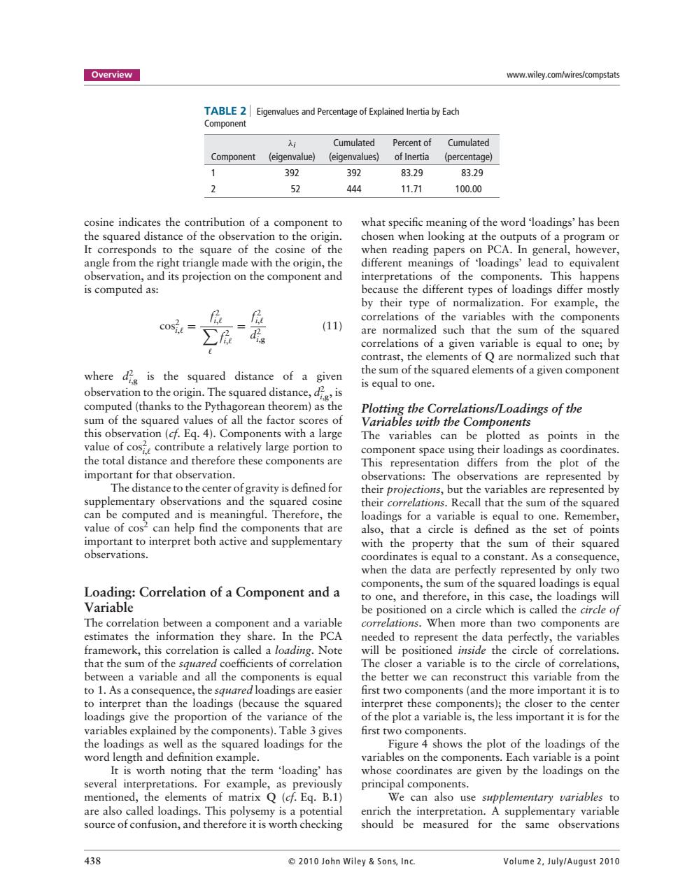
Overview www.wiley.com/wires/compstats TABLE 2 Eigenvalues and Percentage of Explained Inertia by Each Component N Cumulated Percent of Cumulated Component (eigenvalue) (eigenvalues) of Inertia (percentage) 1 392 392 83.29 83.29 2 52 444 11.71 100.00 cosine indicates the contribution of a component to what specific meaning of the word 'loadings'has been the squared distance of the observation to the origin. chosen when looking at the outputs of a program or It corresponds to the square of the cosine of the when reading papers on PCA.In general,however, angle from the right triangle made with the origin,the different meanings of loadings'lead to equivalent observation,and its projection on the component and interpretations of the components.This happens is computed as: because the different types of loadings differ mostly by their type of normalization.For example,the 屁 correlations of the variables with the components (11) are normalized such that the sum of the squared e correlations of a given variable is equal to one;by contrast,the elements of Q are normalized such that where dg is the squared distance of a given the sum of the squared elements of a given component observation to the origin.The squared distance,is is equal to one. computed(thanks to the Pythagorean theorem)as the Plotting the Correlations/Loadings of the sum of the squared values of all the factor scores of Variables with the Components this observation(cf.Eq.4).Components with a large The variables can be plotted as points in the value of cos contribute a relatively large portion to component space using their loadings as coordinates. the total distance and therefore these components are This representation differs from the plot of the important for that observation. observations:The observations are represented by The distance to the center of gravity is defined for their projections,but the variables are represented by supplementary observations and the squared cosine their correlations.Recall that the sum of the squared can be computed and is meaningful.Therefore,the loadings for a variable is equal to one.Remember, value of cos2 can help find the components that are also,that a circle is defined as the set of points important to interpret both active and supplementary with the property that the sum of their squared observations. coordinates is equal to a constant.As a consequence, when the data are perfectly represented by only two components,the sum of the squared loadings is equal Loading:Correlation of a Component and a to one,and therefore,in this case,the loadings will Variable be positioned on a circle which is called the circle of The correlation between a component and a variable correlations.When more than two components are estimates the information they share.In the PCA needed to represent the data perfectly,the variables framework,this correlation is called a loading.Note will be positioned inside the circle of correlations. that the sum of the squared coefficients of correlation The closer a variable is to the circle of correlations, between a variable and all the components is equal the better we can reconstruct this variable from the to 1.As a consequence,the squared loadings are easier first two components(and the more important it is to to interpret than the loadings (because the squared interpret these components);the closer to the center loadings give the proportion of the variance of the of the plot a variable is,the less important it is for the variables explained by the components).Table 3 gives first two components. the loadings as well as the squared loadings for the Figure 4 shows the plot of the loadings of the word length and definition example. variables on the components.Each variable is a point It is worth noting that the term 'loading'has whose coordinates are given by the loadings on the several interpretations.For example,as previously principal components. mentioned,the elements of matrix Q(cf.Eg.B.1) We can also use supplementary variables to are also called loadings.This polysemy is a potential enrich the interpretation.A supplementary variable source of confusion,and therefore it is worth checking should be measured for the same observations 438 2010 John Wiley Sons,Inc. Volume 2,July/August 2010Overview www.wiley.com/wires/compstats TABLE 2 Eigenvalues and Percentage of Explained Inertia by Each Component λi Cumulated Percent of Cumulated Component (eigenvalue) (eigenvalues) of Inertia (percentage) 1 392 392 83.29 83.29 2 52 444 11.71 100.00 cosine indicates the contribution of a component to the squared distance of the observation to the origin. It corresponds to the square of the cosine of the angle from the right triangle made with the origin, the observation, and its projection on the component and is computed as: cos2 i,# = f 2 # i,# # f 2 i,# = f 2 i,# d2 i,g (11) where d2 i,g is the squared distance of a given observation to the origin. The squared distance, d2 i,g, is computed (thanks to the Pythagorean theorem) as the sum of the squared values of all the factor scores of this observation (cf. Eq. 4). Components with a large value of cos2 i,# contribute a relatively large portion to the total distance and therefore these components are important for that observation. The distance to the center of gravity is defined for supplementary observations and the squared cosine can be computed and is meaningful. Therefore, the value of cos2 can help find the components that are important to interpret both active and supplementary observations. Loading: Correlation of a Component and a Variable The correlation between a component and a variable estimates the information they share. In the PCA framework, this correlation is called a loading. Note that the sum of the squared coefficients of correlation between a variable and all the components is equal to 1. As a consequence, the squared loadings are easier to interpret than the loadings (because the squared loadings give the proportion of the variance of the variables explained by the components). Table 3 gives the loadings as well as the squared loadings for the word length and definition example. It is worth noting that the term ‘loading’ has several interpretations. For example, as previously mentioned, the elements of matrix Q (cf. Eq. B.1) are also called loadings. This polysemy is a potential source of confusion, and therefore it is worth checking what specific meaning of the word ‘loadings’ has been chosen when looking at the outputs of a program or when reading papers on PCA. In general, however, different meanings of ‘loadings’ lead to equivalent interpretations of the components. This happens because the different types of loadings differ mostly by their type of normalization. For example, the correlations of the variables with the components are normalized such that the sum of the squared correlations of a given variable is equal to one; by contrast, the elements of Q are normalized such that the sum of the squared elements of a given component is equal to one. Plotting the Correlations/Loadings of the Variables with the Components The variables can be plotted as points in the component space using their loadings as coordinates. This representation differs from the plot of the observations: The observations are represented by their projections, but the variables are represented by their correlations. Recall that the sum of the squared loadings for a variable is equal to one. Remember, also, that a circle is defined as the set of points with the property that the sum of their squared coordinates is equal to a constant. As a consequence, when the data are perfectly represented by only two components, the sum of the squared loadings is equal to one, and therefore, in this case, the loadings will be positioned on a circle which is called the circle of correlations. When more than two components are needed to represent the data perfectly, the variables will be positioned inside the circle of correlations. The closer a variable is to the circle of correlations, the better we can reconstruct this variable from the first two components (and the more important it is to interpret these components); the closer to the center of the plot a variable is, the less important it is for the first two components. Figure 4 shows the plot of the loadings of the variables on the components. Each variable is a point whose coordinates are given by the loadings on the principal components. We can also use supplementary variables to enrich the interpretation. A supplementary variable should be measured for the same observations 438  2010 John Wiley & Son s, In c. Volume 2, July/Augu st 2010