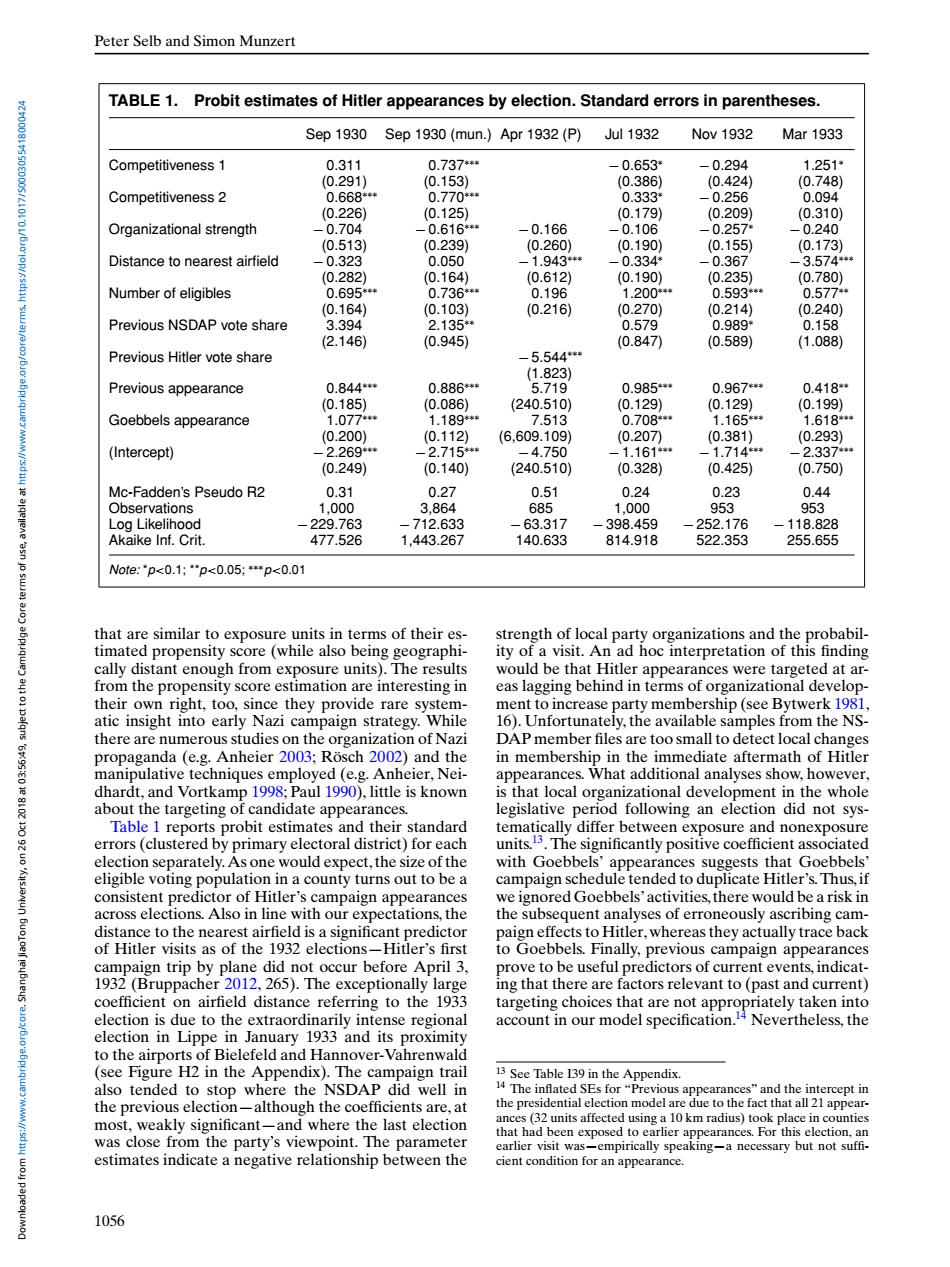
Peter Selb and Simon Munzert TABLE 1. Probit estimates of Hitler appearances by election.Standard errors in parentheses. Sep 1930 Sep 1930(mun.) Apr1932(P) Jul 1932 Nov 1932 Mar 1933 Competitiveness 1 0.311 0.737* -0.653* -0.294 1.251* (0.291) (0.153) (0.386) (0.424) (0.748) Competitiveness 2 0.668* 0.770* 0.333* -0.256 0.094 (0.226) (0.125) (0.179) (0.209) (0.310) Organizational strength -0.704 -0.616* -0.166 -0.106 -0.257* -0.240 (0.513) (0.239) (0.260) (0.190) (0.155) (0.173) Distance to nearest airfield -0.323 0.050 -1.943* -0.334* -0.367 -3.574** (0.282) (0.164) (0.612) (0.190) (0.235) (0.780) Number of eligibles 0.695* 0.736* 0.196 1.200** 0.593* 0.5774 (0.164) (0.103) (0.216) (0.270) (0.214) (0.240) Previous NSDAP vote share 3.394 2.135* 0.579 0.989* 0.158 (2.146) (0.945) (0.847) (0.589) (1.088) Previous Hitler vote share -5.544* (1.823) Previous appearance 0.844** 0.886* 5.719 0.985* 0.967* 0.418 (0.185) (0.086) 240.510) (0.129) (0.129) (0.199) Goebbels appearance 1.077* 1.189* 7.513 0.708* 1.165* 1.618* (0.200) (0.112) (6.609.109) (0.207) (0.381) (0.293) (Intercept) -2.269* -2.715* -4.750 -1.161 -1.714** 2.337* (0.249) (0.140) (240.510) (0.328) (0.425) (0.750) Mc-Fadden's Pseudo R2 0.31 0.27 0.51 0.24 0.23 0.44 Observations 1.000 3.864 685 1.000 953 953 Log Likelihood 229.763 .712.633 63.317 398.459 252.176 118.828 Akaike Inf.Crit. 477.526 1.443.267 140.633 814.918 522.353 255.655 Note:"p<0.1;“p<0.05;**p<0.01 that are similar to exposure units in terms of their es- strength of local party organizations and the probabil- timated propensity score (while also being geographi- ity of a visit.An ad hoc interpretation of this finding cally distant enough from exposure units).The results would be that Hitler appearances were targeted at ar- 是 from the propensity score estimation are interesting in eas lagging behind in terms of organizational develop- their own right,too,since they provide rare system- ment to increase party membership(see Bytwerk 1981 atic insight into early Nazi campaign strategy.While 16).Unfortunately,the available samples from the NS- there are numerous studies on the organization of Nazi DAP member files are too small to detect local changes propaganda(e.g.Anheier 2003;Rosch 2002)and the in membership in the immediate aftermath of Hitler manipulative techniques employed(e.g.Anheier,Nei- appearances.What additional analyses show,however, dhardt,and Vortkamp 1998;Paul 1990),little is known is that local organizational development in the whole about the targeting of candidate appearances. legislative period following an election did not sys- Table 1 reports probit estimates and their standard tematically differ between exposure and nonexposure errors(clustered by primary electoral district)for each units.13.The significantly positive coefficient associated election separately.As one would expect,the size of the with Goebbels'appearances suggests that Goebbels' eligible voting population in a county turns out to be a campaign schedule tended to duplicate Hitler's.Thus,if consistent predictor of Hitler's campaign appearances we ignored Goebbels'activities,there would be a risk in across elections.Also in line with our expectations,the the subsequent analyses of erroneously ascribing cam- distance to the nearest airfield is a significant predictor paign effects to Hitler,whereas they actually trace back of Hitler visits as of the 1932 elections-Hitler's first to Goebbels.Finally,previous campaign appearances campaign trip by plane did not occur before April 3. prove to be useful predictors of current events,indicat- 1932(Bruppacher 2012,265).The exceptionally large ing that there are factors relevant to(past and current) coefficient on airfield distance referring to the 1933 targeting choices that are not appropriately taken into election is due to the extraordinarily intense regional account in our model specification.4 Nevertheless,the election in Lippe in January 1933 and its proximity to the airports of Bielefeld and Hannover-Vahrenwald (see Figure H2 in the Appendix).The campaign trail 13 See Table 139 in the Appendix. also tended to stop where the NSDAP did well in 14 The inflated SEs for"Previous appearances"and the intercept in the previous election-although the coefficients are,at the presidential election model are due to the fact that all 21 appear- most,weakly significant-and where the last election ances(32 units affected using a 10 km radius)took place in counties that had been exposed to earlier appearances.For this election,an was close from the party's viewpoint.The parameter earlier visit was-empirically speaking-a necessary but not suffi- estimates indicate a negative relationship between the cient condition for an appearance. 1056Peter Selb and Simon Munzert TABLE 1. Probit estimates of Hitler appearances by election. Standard errors in parentheses. Sep 1930 Sep 1930 (mun.) Apr 1932 (P) Jul 1932 Nov 1932 Mar 1933 Competitiveness 1 0.311 0.737∗∗∗ − 0.653∗ − 0.294 1.251∗ (0.291) (0.153) (0.386) (0.424) (0.748) Competitiveness 2 0.668∗∗∗ 0.770∗∗∗ 0.333∗ − 0.256 0.094 (0.226) (0.125) (0.179) (0.209) (0.310) Organizational strength − 0.704 − 0.616∗∗∗ − 0.166 − 0.106 − 0.257∗ − 0.240 (0.513) (0.239) (0.260) (0.190) (0.155) (0.173) Distance to nearest airfield − 0.323 0.050 − 1.943∗∗∗ − 0.334∗ − 0.367 − 3.574∗∗∗ (0.282) (0.164) (0.612) (0.190) (0.235) (0.780) Number of eligibles 0.695∗∗∗ 0.736∗∗∗ 0.196 1.200∗∗∗ 0.593∗∗∗ 0.577∗∗ (0.164) (0.103) (0.216) (0.270) (0.214) (0.240) Previous NSDAP vote share 3.394 2.135∗∗ 0.579 0.989∗ 0.158 (2.146) (0.945) (0.847) (0.589) (1.088) Previous Hitler vote share − 5.544∗∗∗ (1.823) Previous appearance 0.844∗∗∗ 0.886∗∗∗ 5.719 0.985∗∗∗ 0.967∗∗∗ 0.418∗∗ (0.185) (0.086) (240.510) (0.129) (0.129) (0.199) Goebbels appearance 1.077∗∗∗ 1.189∗∗∗ 7.513 0.708∗∗∗ 1.165∗∗∗ 1.618∗∗∗ (0.200) (0.112) (6,609.109) (0.207) (0.381) (0.293) (Intercept) − 2.269∗∗∗ − 2.715∗∗∗ − 4.750 − 1.161∗∗∗ − 1.714∗∗∗ − 2.337∗∗∗ (0.249) (0.140) (240.510) (0.328) (0.425) (0.750) Mc-Fadden’s Pseudo R2 0.31 0.27 0.51 0.24 0.23 0.44 Observations 1,000 3,864 685 1,000 953 953 Log Likelihood − 229.763 − 712.633 − 63.317 − 398.459 − 252.176 − 118.828 Akaike Inf. Crit. 477.526 1,443.267 140.633 814.918 522.353 255.655 Note: *p<0.1; **p<0.05; ∗∗∗p<0.01 that are similar to exposure units in terms of their es￾timated propensity score (while also being geographi￾cally distant enough from exposure units). The results from the propensity score estimation are interesting in their own right, too, since they provide rare system￾atic insight into early Nazi campaign strategy. While there are numerous studies on the organization of Nazi propaganda (e.g. Anheier 2003; Rösch 2002) and the manipulative techniques employed (e.g. Anheier, Nei￾dhardt, and Vortkamp 1998; Paul 1990), little is known about the targeting of candidate appearances. Table 1 reports probit estimates and their standard errors (clustered by primary electoral district) for each election separately.As one would expect, the size of the eligible voting population in a county turns out to be a consistent predictor of Hitler’s campaign appearances across elections. Also in line with our expectations, the distance to the nearest airfield is a significant predictor of Hitler visits as of the 1932 elections—Hitler’s first campaign trip by plane did not occur before April 3, 1932 (Bruppacher 2012, 265). The exceptionally large coefficient on airfield distance referring to the 1933 election is due to the extraordinarily intense regional election in Lippe in January 1933 and its proximity to the airports of Bielefeld and Hannover-Vahrenwald (see Figure H2 in the Appendix). The campaign trail also tended to stop where the NSDAP did well in the previous election—although the coefficients are, at most, weakly significant—and where the last election was close from the party’s viewpoint. The parameter estimates indicate a negative relationship between the strength of local party organizations and the probabil￾ity of a visit. An ad hoc interpretation of this finding would be that Hitler appearances were targeted at ar￾eas lagging behind in terms of organizational develop￾ment to increase party membership (see Bytwerk 1981, 16). Unfortunately, the available samples from the NS￾DAP member files are too small to detect local changes in membership in the immediate aftermath of Hitler appearances. What additional analyses show, however, is that local organizational development in the whole legislative period following an election did not sys￾tematically differ between exposure and nonexposure units.13. The significantly positive coefficient associated with Goebbels’ appearances suggests that Goebbels’ campaign schedule tended to duplicate Hitler’s.Thus,if we ignored Goebbels’ activities, there would be a risk in the subsequent analyses of erroneously ascribing cam￾paign effects to Hitler, whereas they actually trace back to Goebbels. Finally, previous campaign appearances prove to be useful predictors of current events, indicat￾ing that there are factors relevant to (past and current) targeting choices that are not appropriately taken into account in our model specification.14 Nevertheless, the 13 See Table I39 in the Appendix. 14 The inflated SEs for “Previous appearances” and the intercept in the presidential election model are due to the fact that all 21 appear￾ances (32 units affected using a 10 km radius) took place in counties that had been exposed to earlier appearances. For this election, an earlier visit was—empirically speaking—a necessary but not suffi￾cient condition for an appearance. 1056 Downloaded from https://www.cambridge.org/core. Shanghai JiaoTong University, on 26 Oct 2018 at 03:56:49, subject to the Cambridge Core terms of use, available at https://www.cambridge.org/core/terms. https://doi.org/10.1017/S0003055418000424