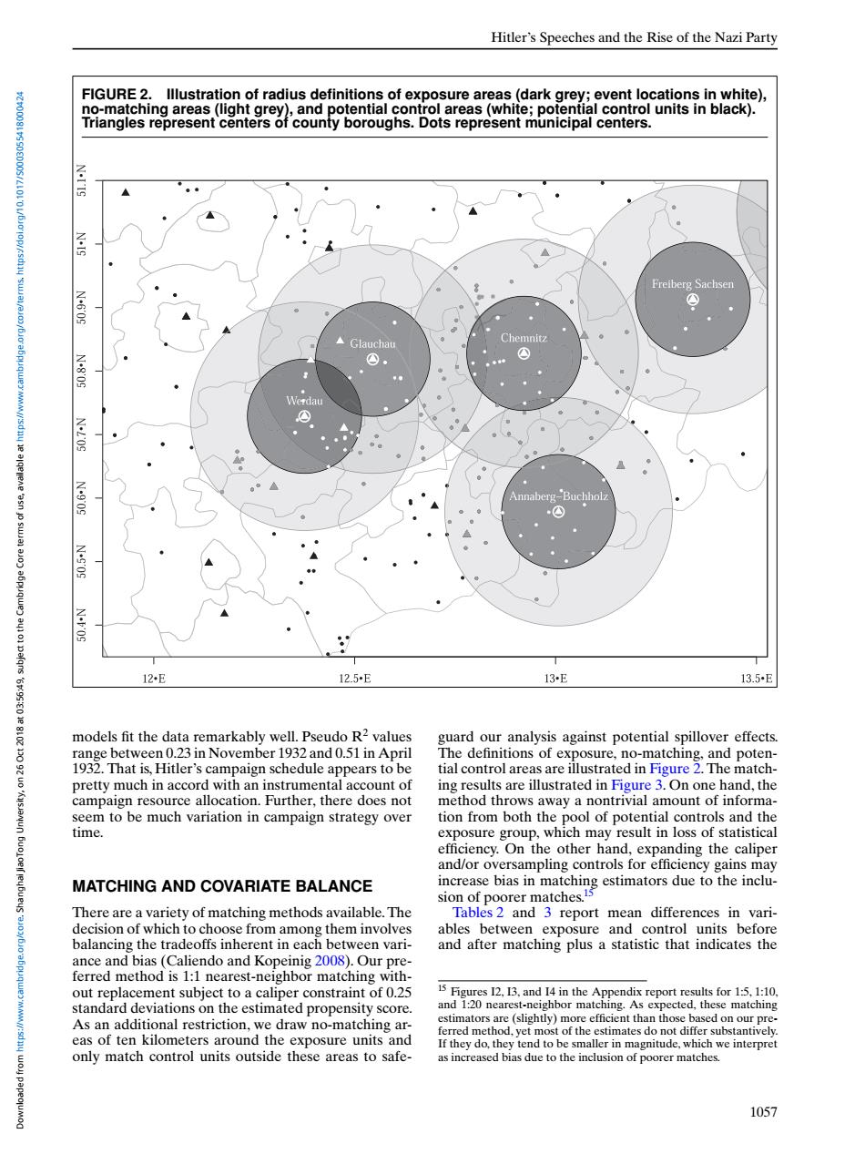
Hitler's Speeches and the Rise of the Nazi Party FIGURE 2.Illustration of radius definitions of exposure areas(dark grey;event locations in white), no-matching areas(light grey),and potential control areas(white;potential control units in black). Triangles represent centers of county boroughs.Dots represent municipal centers. N.T Freiberg Sachsen N.609 0 ▲Glauchau Chemnitz ⊙· © Werdau 4号 。 Annaberg-Buchholz ④ 4905 N+F'OS 12-E 12.5-E 13-E 13.5-E models fit the data remarkably well.Pseudo R2 values guard our analysis against potential spillover effects. range between 0.23 in November 1932 and 0.51 in April The definitions of exposure,no-matching,and poten- 1932.That is,Hitler's campaign schedule appears to be tial control areas are illustrated in Figure 2.The match- pretty much in accord with an instrumental account of ing results are illustrated in Figure 3.On one hand,the campaign resource allocation.Further,there does not method throws away a nontrivial amount of informa seem to be much variation in campaign strategy over tion from both the pool of potential controls and the time. exposure group,which may result in loss of statistical efficiency.On the other hand,expanding the caliper and/or oversampling controls for efficiency gains may MATCHING AND COVARIATE BALANCE increase bias in matching estimators due to the inclu- sion of poorer matches.15 There are a variety of matching methods available.The Tables 2 and 3 report mean differences in vari- decision of which to choose from among them involves ables between exposure and control units before balancing the tradeoffs inherent in each between vari- and after matching plus a statistic that indicates the ance and bias(Caliendo and Kopeinig 2008).Our pre- ferred method is 1:1 nearest-neighbor matching with- out replacement subject to a caliper constraint of 0.25 15 Figures 12.13.and 14 in the Appendix report results for 1:5,1:10. standard deviations on the estimated propensity score. and 1:20 nearest-neighbor matching.As expected,these matching As an additional restriction,we draw no-matching ar- estimators are(slightly)more efficient than those based on our pre- ferred method,yet most of the estimates do not differ substantively eas of ten kilometers around the exposure units and If they do,they tend to be smaller in magnitude,which we interpret only match control units outside these areas to safe- as increased bias due to the inclusion of poorer matches. 1057Hitler’s Speeches and the Rise of the Nazi Party FIGURE 2. Illustration of radius definitions of exposure areas (dark grey; event locations in white), no-matching areas (light grey), and potential control areas (white; potential control units in black). Triangles represent centers of county boroughs. Dots represent municipal centers. models fit the data remarkably well. Pseudo R2 values range between 0.23 in November 1932 and 0.51 in April 1932. That is, Hitler’s campaign schedule appears to be pretty much in accord with an instrumental account of campaign resource allocation. Further, there does not seem to be much variation in campaign strategy over time. MATCHING AND COVARIATE BALANCE There are a variety of matching methods available. The decision of which to choose from among them involves balancing the tradeoffs inherent in each between vari￾ance and bias (Caliendo and Kopeinig 2008). Our pre￾ferred method is 1:1 nearest-neighbor matching with￾out replacement subject to a caliper constraint of 0.25 standard deviations on the estimated propensity score. As an additional restriction, we draw no-matching ar￾eas of ten kilometers around the exposure units and only match control units outside these areas to safe￾guard our analysis against potential spillover effects. The definitions of exposure, no-matching, and poten￾tial control areas are illustrated in Figure 2. The match￾ing results are illustrated in Figure 3. On one hand, the method throws away a nontrivial amount of informa￾tion from both the pool of potential controls and the exposure group, which may result in loss of statistical efficiency. On the other hand, expanding the caliper and/or oversampling controls for efficiency gains may increase bias in matching estimators due to the inclu￾sion of poorer matches.15 Tables 2 and 3 report mean differences in vari￾ables between exposure and control units before and after matching plus a statistic that indicates the 15 Figures I2, I3, and I4 in the Appendix report results for 1:5, 1:10, and 1:20 nearest-neighbor matching. As expected, these matching estimators are (slightly) more efficient than those based on our pre￾ferred method, yet most of the estimates do not differ substantively. If they do, they tend to be smaller in magnitude, which we interpret as increased bias due to the inclusion of poorer matches. 1057 Downloaded from https://www.cambridge.org/core. Shanghai JiaoTong University, on 26 Oct 2018 at 03:56:49, subject to the Cambridge Core terms of use, available at https://www.cambridge.org/core/terms. https://doi.org/10.1017/S0003055418000424