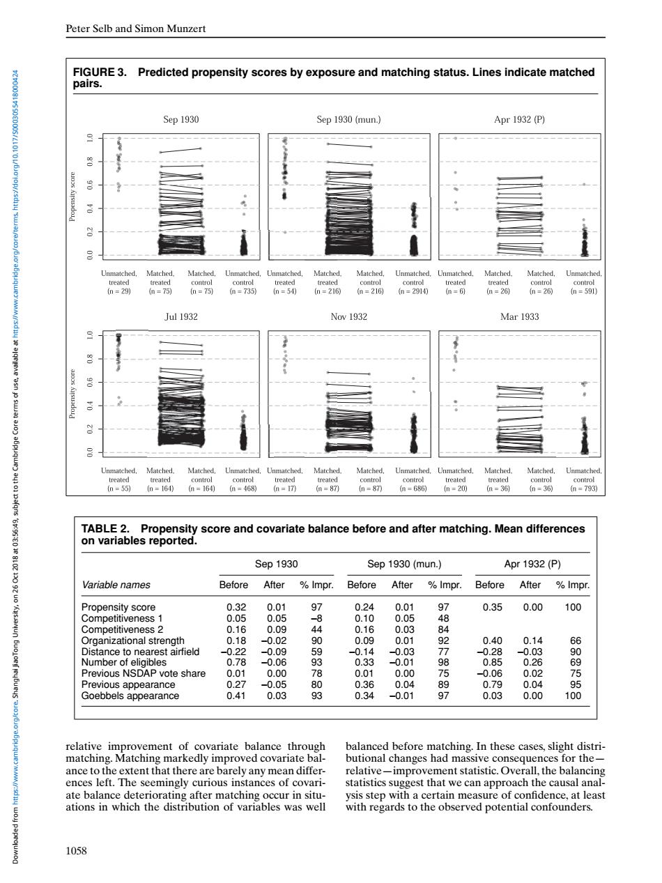
Peter Selb and Simon Munzert FIGURE 3.Predicted propensity scores by exposure and matching status.Lines indicate matched pairs. Sep 1930 Sep 1930(mun.) Apr1932(P) Unmatched.Matched Matched.Unmatched,Unmatched,Matched. Matched. Unmatched.Unmatched.Matched. Matched. Unmatched trealed trealed control control treated trealed contol control treated treated contro control (n=29) =75 (n=75) =7350 n=54) (n=216份 (0=216m=2914) n=6 (0=26 n=26粉 (n=591) Jul 1932 Nov 1932 Mar 1933 上一 Unmatched.Matched. Matched, Unmatched,Unmatched, Matched. Matched, Unmatched,Unmatched, Matched. Matched, Unmatched treated treated control control treated control control treated treated control control h=55) n=164 (=16) (n=468) (a=170 m=87 (n=87) (=686) (n=20) (n=36 n=36) (=793) TABLE 2. Propensity score and covariate balance before and after matching.Mean differences on variables reported. Sep 1930 Sep 1930(mun.) Apr1932(P) Variable names Before After Impr. Before After Impr. Before After Impr Propensity score 0.32 0.01 97 0.24 0.01 97 0.35 0.00 100 Competitiveness 1 0.05 0.05 -8 0.10 0.05 48 Competitiveness 2 0.16 0.09 44 0.16 0.03 Organizational strength 0.18 -0.02 90 0.09 0.01 92 0.40 0.14 6 Distance to nearest airfield -0.22 -0.09 9 -0.14 0.03 -0.28 -0.03 0 Number of eligibles 0.78 -0.06 9 0.33 -0.01 98 0.85 0.26 69 Previous NSDAP vote share 0.01 0.00 78 0.01 0.00 -0.06 0.02 Previous appearance 0.27 -0.05 0.36 0.04 0.79 0.04 95 Goebbels appearance 0.41 0.03 93 0.34 -0.01 97 0.03 0.00 100 relative improvement of covariate balance through balanced before matching.In these cases,slight distri- matching.Matching markedly improved covariate bal- butional changes had massive consequences for the- ance to the extent that there are barely any mean differ- relative-improvement statistic.Overall,the balancing ences left.The seemingly curious instances of covari- statistics suggest that we can approach the causal anal- ate balance deteriorating after matching occur in situ- ysis step with a certain measure of confidence,at least ations in which the distribution of variables was well with regards to the observed potential confounders. 1058Peter Selb and Simon Munzert FIGURE 3. Predicted propensity scores by exposure and matching status. Lines indicate matched pairs. TABLE 2. Propensity score and covariate balance before and after matching. Mean differences on variables reported. Sep 1930 Sep 1930 (mun.) Apr 1932 (P) Variable names Before After % Impr. Before After % Impr. Before After % Impr. Propensity score 0.32 0.01 97 0.24 0.01 97 0.35 0.00 100 Competitiveness 1 0.05 0.05 –8 0.10 0.05 48 Competitiveness 2 0.16 0.09 44 0.16 0.03 84 Organizational strength 0.18 –0.02 90 0.09 0.01 92 0.40 0.14 66 Distance to nearest airfield –0.22 –0.09 59 –0.14 –0.03 77 –0.28 –0.03 90 Number of eligibles 0.78 –0.06 93 0.33 –0.01 98 0.85 0.26 69 Previous NSDAP vote share 0.01 0.00 78 0.01 0.00 75 –0.06 0.02 75 Previous appearance 0.27 –0.05 80 0.36 0.04 89 0.79 0.04 95 Goebbels appearance 0.41 0.03 93 0.34 –0.01 97 0.03 0.00 100 relative improvement of covariate balance through matching. Matching markedly improved covariate bal￾ance to the extent that there are barely any mean differ￾ences left. The seemingly curious instances of covari￾ate balance deteriorating after matching occur in situ￾ations in which the distribution of variables was well balanced before matching. In these cases, slight distri￾butional changes had massive consequences for the— relative—improvement statistic. Overall, the balancing statistics suggest that we can approach the causal anal￾ysis step with a certain measure of confidence, at least with regards to the observed potential confounders. 1058 Downloaded from https://www.cambridge.org/core. Shanghai JiaoTong University, on 26 Oct 2018 at 03:56:49, subject to the Cambridge Core terms of use, available at https://www.cambridge.org/core/terms. https://doi.org/10.1017/S0003055418000424