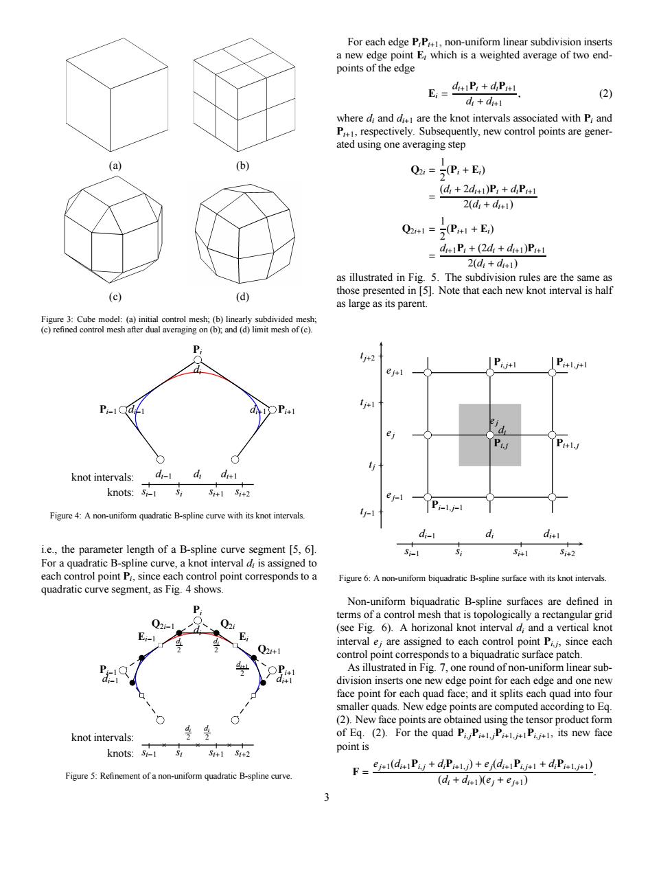
E-+ 0=B+ r 下4Aaa山ai:B-oplire cuv with】 New ed (2)F(a) (b) (c) (d) Figure 3: Cube model: (a) initial control mesh; (b) linearly subdivided mesh; (c) refined control mesh after dual averaging on (b); and (d) limit mesh of (c). bc bc bc bc bc Pi Pi−1 Pi+1 di di−1 di+1 | | | | si−1 si si+1 si+2 knot intervals: di−1 di di+1 knots: Figure 4: A non-uniform quadratic B-spline curve with its knot intervals. i.e., the parameter length of a B-spline curve segment [5, 6]. For a quadratic B-spline curve, a knot interval di is assigned to each control point Pi , since each control point corresponds to a quadratic curve segment, as Fig. 4 shows. bc bc bc bc bc b b b b b b rs rs rs rs Pi Pi−1 Pi+1 di di−1 di+1 Ei−1 Ei Q2i−1 Q2i Q2i+1 di 2 di 2 di+1 2 | | | | si−1 si si+1 si+2 di 2 di 2 × × × knot intervals: knots: Figure 5: Refinement of a non-uniform quadratic B-spline curve. For each edge PiPi+1, non-uniform linear subdivision inserts a new edge point Ei which is a weighted average of two end￾points of the edge Ei = di+1Pi + diPi+1 di + di+1 , (2) where di and di+1 are the knot intervals associated with Pi and Pi+1, respectively. Subsequently, new control points are gener￾ated using one averaging step Q2i = 1 2 (Pi + Ei) = (di + 2di+1)Pi + diPi+1 2(di + di+1) Q2i+1 = 1 2 (Pi+1 + Ei) = di+1Pi + (2di + di+1)Pi+1 2(di + di+1) as illustrated in Fig. 5. The subdivision rules are the same as those presented in [5]. Note that each new knot interval is half as large as its parent. bc bc bc bc bc bc bc bc bc Pi, j di ej Pi+1, j Pi, j+1 Pi+1, j+1 Pi−1, j−1 | | | | si−1 si si+1 si+2 di−1 di di+1 + + + + tj−1 tj tj+1 tj+2 ej−1 ej ej+1 Figure 6: A non-uniform biquadratic B-spline surface with its knot intervals. Non-uniform biquadratic B-spline surfaces are defined in terms of a control mesh that is topologically a rectangular grid (see Fig. 6). A horizonal knot interval di and a vertical knot interval ej are assigned to each control point Pi, j , since each control point corresponds to a biquadratic surface patch. As illustrated in Fig. 7, one round of non-uniform linear sub￾division inserts one new edge point for each edge and one new face point for each quad face; and it splits each quad into four smaller quads. New edge points are computed according to Eq. (2). New face points are obtained using the tensor product form of Eq. (2). For the quad Pi, jPi+1, jPi+1, j+1Pi, j+1, its new face point is F = ej+1(di+1Pi, j + diPi+1, j) + ej(di+1Pi, j+1 + diPi+1, j+1) (di + di+1)(ej + ej+1) . 3