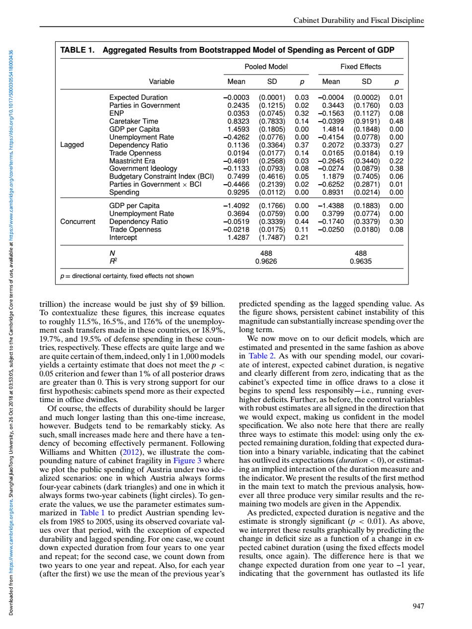
Cabinet Durability and Fiscal Discipline TABLE 1.Aggregated Results from Bootstrapped Model of Spending as Percent of GDP Pooled Model Fixed Effects Variable Mean SD p Mean SD p Expected Duration -0.0003 (0.0001) 0.03 -0.0004 0.0002) 0.01 Parties in Government 0.2435 (0.1215) 0.02 0.3443 (0.1760) 0.03 ENP 0.0353 (0.0745) 0.32 -0.1563 (0.1127) 0.08 Caretaker Time 0.8323 (0.7833) 0.14 0.0399 (0.9191) 0.48 GDP per Capita 1.4593 (0.1805) 0.00 1.4814 (0.1848) 0.00 Unemployment Rate -0.4262 (0.0776) 0.00 0.4154 (0.0778) 0.00 Lagged Dependency Ratio 0.1136 (0.3364) 0.37 0.2072 (0.3373) 0.27 Trade Openness 0.0194 (0.0177) 0.14 0.0165 (0.0184) 0.19 Maastricht Era -0.4691 (0.2568) 0.03 -0.2645 0.3440) 0.22 Government Ideology -0.1133 (0.0793) 0.08 _0.0274 (0.0879) 0.38 Budgetary Constraint Index(BCI) 0.7499 (0.4616) 0.05 1.1879 (0.7405) 0.06 Parties in Government x BCI _0.4466 0.2139 0.02 -0.6252 (0.2871) 0.01 Spending 0.9295 0.0112) 0.00 0.8931 (0.0214) 0.00 GDP per Capita -1.4092 (0.1766) 0.00 -1.4388 (0.1883) 0.00 Unemployment Rate 0.3694 (0.0759) 0.00 0.3799 (0.0774) 0.00 Concurrent Dependency Ratio 0.0519 (0.3339) 0.44 0.1740 (0.3379) 0.30 Trade Openness -0.0218 (0.0175 0.11 0.0250 (0.0180) 0.08 Intercept 1.4287 (1.7487) 0.21 4号元 N 488 488 0.9626 0.9635 'asn p=directional certainty,fixed effects not shown trillion)the increase would be just shy of $9 billion predicted spending as the lagged spending value.As To contextualize these figures,this increase equates the figure shows,persistent cabinet instability of this to roughly 11.5%,16.5%,and 176%of the unemploy- magnitude can substantially increase spending over the ment cash transfers made in these countries,or 18.9%. long term. 是 19.7%,and 19.5%of defense spending in these coun- We now move on to our deficit models,which are tries,respectively.These effects are quite large and we estimated and presented in the same fashion as above are quite certain of them,indeed,only 1 in 1,000 models in Table 2.As with our spending model,our covari- yields a certainty estimate that does not meet the p< ate of interest,expected cabinet duration,is negative 0.05 criterion and fewer than 1%of all posterior draws and clearly different from zero,indicating that as the are greater than 0.This is very strong support for our cabinet's expected time in office draws to a close it first hypothesis:cabinets spend more as their expected begins to spend less responsibly-i.e..running ever- time in office dwindles. higher deficits.Further,as before,the control variables Of course,the effects of durability should be larger with robust estimates are all signed in the direction that and much longer lasting than this one-time increase. we would expect,making us confident in the model however.Budgets tend to be remarkably sticky.As specification.We also note here that there are really such,small increases made here and there have a ten- three ways to estimate this model:using only the ex- dency of becoming effectively permanent.Following pected remaining duration,folding that expected dura- Williams and Whitten (2012),we illustrate the com- tion into a binary variable,indicating that the cabinet pounding nature of cabinet fragility in Figure 3 where has outlived its expectations(duration <0),or estimat- we plot the public spending of Austria under two ide- ing an implied interaction of the duration measure and alized scenarios:one in which Austria always forms the indicator.We present the results of the first method four-year cabinets (dark triangles)and one in which it in the main text to match the previous analysis,how- always forms two-year cabinets (light circles).To gen- ever all three produce very similar results and the re- erate the values,we use the parameter estimates sum- maining two models are given in the Appendix. marized in Table 1 to predict Austrian spending lev- As predicted,expected duration is negative and the els from 1985 to 2005.using its observed covariate val- estimate is strongly significant (p <0.01).As above. ues over that period,with the exception of expected we interpret these results graphically by predicting the durability and lagged spending.For one case,we count change in deficit size as a function of a change in ex- down expected duration from four years to one year pected cabinet duration(using the fixed effects model and repeat;for the second case,we count down from results,once again).The difference here is that we two years to one year and repeat.Also,for each year change expected duration from one year to-1 year, (after the first)we use the mean of the previous year's indicating that the government has outlasted its life 947Cabinet Durability and Fiscal Discipline TABLE 1. Aggregated Results from Bootstrapped Model of Spending as Percent of GDP Pooled Model Fixed Effects Variable Mean SD p Mean SD p Lagged Expected Duration –0.0003 (0.0001) 0.03 –0.0004 (0.0002) 0.01 Parties in Government 0.2435 (0.1215) 0.02 0.3443 (0.1760) 0.03 ENP 0.0353 (0.0745) 0.32 –0.1563 (0.1127) 0.08 Caretaker Time 0.8323 (0.7833) 0.14 –0.0399 (0.9191) 0.48 GDP per Capita 1.4593 (0.1805) 0.00 1.4814 (0.1848) 0.00 Unemployment Rate –0.4262 (0.0776) 0.00 –0.4154 (0.0778) 0.00 Dependency Ratio 0.1136 (0.3364) 0.37 0.2072 (0.3373) 0.27 Trade Openness 0.0194 (0.0177) 0.14 0.0165 (0.0184) 0.19 Maastricht Era –0.4691 (0.2568) 0.03 –0.2645 (0.3440) 0.22 Government Ideology –0.1133 (0.0793) 0.08 –0.0274 (0.0879) 0.38 Budgetary Constraint Index (BCI) 0.7499 (0.4616) 0.05 1.1879 (0.7405) 0.06 Parties in Government × BCI –0.4466 (0.2139) 0.02 –0.6252 (0.2871) 0.01 Spending 0.9295 (0.0112) 0.00 0.8931 (0.0214) 0.00 Concurrent GDP per Capita –1.4092 (0.1766) 0.00 –1.4388 (0.1883) 0.00 Unemployment Rate 0.3694 (0.0759) 0.00 0.3799 (0.0774) 0.00 Dependency Ratio –0.0519 (0.3339) 0.44 –0.1740 (0.3379) 0.30 Trade Openness –0.0218 (0.0175) 0.11 –0.0250 (0.0180) 0.08 Intercept 1.4287 (1.7487) 0.21 N 488 488 R2 0.9626 0.9635 p = directional certainty, fixed effects not shown trillion) the increase would be just shy of $9 billion. To contextualize these figures, this increase equates to roughly 11.5%, 16.5%, and 17.6% of the unemploy￾ment cash transfers made in these countries, or 18.9%, 19.7%, and 19.5% of defense spending in these coun￾tries, respectively. These effects are quite large and we are quite certain of them,indeed, only 1 in 1,000 models yields a certainty estimate that does not meet the p < 0.05 criterion and fewer than 1% of all posterior draws are greater than 0. This is very strong support for our first hypothesis: cabinets spend more as their expected time in office dwindles. Of course, the effects of durability should be larger and much longer lasting than this one-time increase, however. Budgets tend to be remarkably sticky. As such, small increases made here and there have a ten￾dency of becoming effectively permanent. Following Williams and Whitten (2012), we illustrate the com￾pounding nature of cabinet fragility in Figure 3 where we plot the public spending of Austria under two ide￾alized scenarios: one in which Austria always forms four-year cabinets (dark triangles) and one in which it always forms two-year cabinets (light circles). To gen￾erate the values, we use the parameter estimates sum￾marized in Table 1 to predict Austrian spending lev￾els from 1985 to 2005, using its observed covariate val￾ues over that period, with the exception of expected durability and lagged spending. For one case, we count down expected duration from four years to one year and repeat; for the second case, we count down from two years to one year and repeat. Also, for each year (after the first) we use the mean of the previous year’s predicted spending as the lagged spending value. As the figure shows, persistent cabinet instability of this magnitude can substantially increase spending over the long term. We now move on to our deficit models, which are estimated and presented in the same fashion as above in Table 2. As with our spending model, our covari￾ate of interest, expected cabinet duration, is negative and clearly different from zero, indicating that as the cabinet’s expected time in office draws to a close it begins to spend less responsibly—i.e., running ever￾higher deficits. Further, as before, the control variables with robust estimates are all signed in the direction that we would expect, making us confident in the model specification. We also note here that there are really three ways to estimate this model: using only the ex￾pected remaining duration, folding that expected dura￾tion into a binary variable, indicating that the cabinet has outlived its expectations (duration < 0), or estimat￾ing an implied interaction of the duration measure and the indicator.We present the results of the first method in the main text to match the previous analysis, how￾ever all three produce very similar results and the re￾maining two models are given in the Appendix. As predicted, expected duration is negative and the estimate is strongly significant (p < 0.01). As above, we interpret these results graphically by predicting the change in deficit size as a function of a change in ex￾pected cabinet duration (using the fixed effects model results, once again). The difference here is that we change expected duration from one year to –1 year, indicating that the government has outlasted its life 947 Downloaded from https://www.cambridge.org/core. Shanghai JiaoTong University, on 26 Oct 2018 at 03:53:05, subject to the Cambridge Core terms of use, available at https://www.cambridge.org/core/terms. https://doi.org/10.1017/S0003055418000436