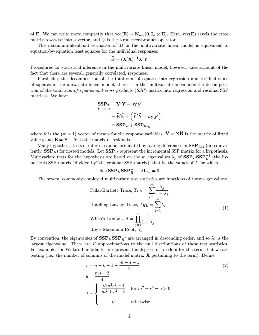
of E.We can write more compactly that vec(E)~Nnm(0,In )Here,vec(E)ravels the error matrix row-wise into a vector,and is the Kronecker-product operator. The maximum-likelihood estimator of B in the multivariate linear model is equivalent to equation-by-equation least squares for the individual responses: B=(X'X)-X'Y Procedures for statistical inference in the multivariate linear model,however,take account of the fact that there are several,generally correlated,responses. Paralleling the decomposition of the total sum of squares into regression and residual sums of squares in the univariate linear model,there is in the multivariate linear model a decomposi- tion of the total sum-of-squares-and-cross-products (SSP)matrix into regression and residual SSP matrices.We have SSPT Y'Y-nyy (m×m) =它+(Y'空-n寸） SSPR+SSPReg where y is the (m x 1)vector of means for the response variables;Y=XB is the matrix of fitted values;and E=Y-Y is the matrix of residuals. Many hypothesis tests of interest can be formulated by taking differences in SSPReg(or,equiva- lently,SSPR)for nested models.Let SSPH represent the incremental SSP matrix for a hypothesis. Multivariate tests for the hypothesis are based on the m eigenvalues of SSPrSSP(the hy- pothesis SSP matrix"divided by"the residual SSP matrix),that is,the values of A for which det(SSPHSSPR-AI)=0 The several commonly employed multivariate test statistics are functions of these eigenvalues: llai-Bartlett Trace,TP=A m Hotelling-Lawley Trace,T=j j=1 (1) m 1 Wilks's Lambda,A= j=1 Roy's Maximum Root,Ai By convention,the eigenvalues of SSPHSSPR are arranged in descending order,and so is the largest eigenvalue.There are F approximations to the null distributions of these test statistics. For example,for Wilks's Lambda,let s represent the degrees of freedom for the term that we are testing (i.e.,the number of columns of the model matrix X pertaining to the term).Define r=n-k-1-m-8+1 2 (2) u=ms-2 4 Vm2s2-4 m2+s2-5 for m2+s2-5>0 t 0 otherwise 2of E. We can write more compactly that vec(E) ∼ Nnm(0, In ⊗ Σ). Here, vec(E) ravels the error matrix row-wise into a vector, and ⊗ is the Kronecker-product operator. The maximum-likelihood estimator of B in the multivariate linear model is equivalent to equation-by-equation least squares for the individual responses: Bb = (X0X) −1X0Y Procedures for statistical inference in the multivariate linear model, however, take account of the fact that there are several, generally correlated, responses. Paralleling the decomposition of the total sum of squares into regression and residual sums of squares in the univariate linear model, there is in the multivariate linear model a decomposi￾tion of the total sum-of-squares-and-cross-products (SSP) matrix into regression and residual SSP matrices. We have SSPT (m×m) = Y0Y − ny y 0 = Eb0Eb +  Yb 0Yb − ny y 0  = SSPR + SSPReg where y is the (m × 1) vector of means for the response variables; Yb = XBb is the matrix of fitted values; and Eb = Y − Yb is the matrix of residuals. Many hypothesis tests of interest can be formulated by taking differences in SSPReg (or, equiva￾lently, SSPR) for nested models. Let SSPH represent the incremental SSP matrix for a hypothesis. Multivariate tests for the hypothesis are based on the m eigenvalues λj of SSPHSSP−1 R (the hy￾pothesis SSP matrix “divided by” the residual SSP matrix), that is, the values of λ for which det(SSPHSSP−1 R − λIm) = 0 The several commonly employed multivariate test statistics are functions of these eigenvalues: Pillai-Bartlett Trace, TP B = Xm j=1 λj 1 − λj Hotelling-Lawley Trace, THL = Xm j=1 λj Wilks’s Lambda, Λ = Ym j=1 1 1 + λj Roy’s Maximum Root, λ1 (1) By convention, the eigenvalues of SSPHSSP−1 R are arranged in descending order, and so λ1 is the largest eigenvalue. There are F approximations to the null distributions of these test statistics. For example, for Wilks’s Lambda, let s represent the degrees of freedom for the term that we are testing (i.e., the number of columns of the model matrix X pertaining to the term). Define r = n − k − 1 − m − s + 1 2 (2) u = ms − 2 4 t =    √ m2s 2 − 4 m2 + s 2 − 5 for m2 + s 2 − 5 > 0 0 otherwise 2