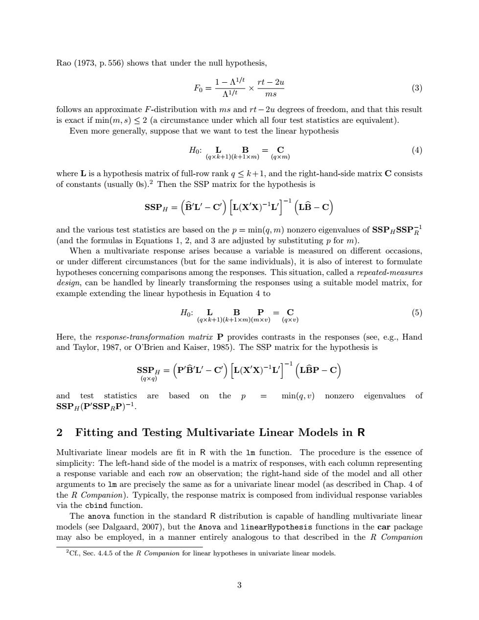
Rao (1973,p.556)shows that under the null hypothesis, 1-△1/trt-2u F0= 41/× (3) ms follows an approximate F-distribution with ms and rt-2u degrees of freedom,and that this result is exact if min(m,s)<2(a circumstance under which all four test statistics are equivalent). Even more generally,suppose that we want to test the linear hypothesis Ho:L B=C (4) (g×k+1)(k+1×m)(q×m) where L is a hypothesis matrix of full-row rank g<k+1,and the right-hand-side matrix C consists of constants(usually 0s).2 Then the SSP matrix for the hypothesis is SSP=(B-C)L(X')L](LB-c) and the various test statistics are based on the p=min(g,m)nonzero eigenvalues of SSPSSPR (and the formulas in Equations 1,2,and 3 are adjusted by substituting p for m) When a multivariate response arises because a variable is measured on different occasions, or under different circumstances (but for the same individuals),it is also of interest to formulate hypotheses concerning comparisons among the responses.This situation,called a repeated-measures design,can be handled by linearly transforming the responses using a suitable model matrix,for example extending the linear hypothesis in Equation 4 to Ho:L B P =C (5) (g×k+1)(k+1×m)(m×v)(9×u) Here,the response-transformation matrix P provides contrasts in the responses (see,e.g.,Hand and Taylor,1987,or O'Brien and Kaiser,1985).The SSP matrix for the hypothesis is SSPa=(P'BL-CL(X'x)L LBP-C) (gxq） and test statistics are based on the p=min(g,v) nonzero eigenvalues of SSPH(P'SSPRP)-1. 2 Fitting and Testing Multivariate Linear Models in R Multivariate linear models are fit in R with the lm function.The procedure is the essence of simplicity:The left-hand side of the model is a matrix of responses,with each column representing a response variable and each row an observation;the right-hand side of the model and all other arguments to lm are precisely the same as for a univariate linear model (as described in Chap.4 of the R Companion).Typically,the response matrix is composed from individual response variables via the cbind function. The anova function in the standard R distribution is capable of handling multivariate linear models(see Dalgaard,2007),but the Anova and linearHypothesis functions in the car package may also be employed,in a manner entirely analogous to that described in the R Companion 2Cf.,Sec.4.4.5 of the R Companion for linear hypotheses in univariate linear models. 3Rao (1973, p. 556) shows that under the null hypothesis, F0 = 1 − Λ 1/t Λ1/t × rt − 2u ms (3) follows an approximate F-distribution with ms and rt−2u degrees of freedom, and that this result is exact if min(m, s) ≤ 2 (a circumstance under which all four test statistics are equivalent). Even more generally, suppose that we want to test the linear hypothesis H0: L (q×k+1) B (k+1×m) = C (q×m) (4) where L is a hypothesis matrix of full-row rank q ≤ k+1, and the right-hand-side matrix C consists of constants (usually 0s).2 Then the SSP matrix for the hypothesis is SSPH =  Bb0L 0 − C0  hL(X 0X) −1L 0 i−1  LBb − C  and the various test statistics are based on the p = min(q, m) nonzero eigenvalues of SSPHSSP−1 R (and the formulas in Equations 1, 2, and 3 are adjusted by substituting p for m). When a multivariate response arises because a variable is measured on different occasions, or under different circumstances (but for the same individuals), it is also of interest to formulate hypotheses concerning comparisons among the responses. This situation, called a repeated-measures design, can be handled by linearly transforming the responses using a suitable model matrix, for example extending the linear hypothesis in Equation 4 to H0: L (q×k+1) B (k+1×m) P (m×v) = C (q×v) (5) Here, the response-transformation matrix P provides contrasts in the responses (see, e.g., Hand and Taylor, 1987, or O’Brien and Kaiser, 1985). The SSP matrix for the hypothesis is SSPH (q×q) =  P 0Bb0L 0 − C0  hL(X 0X) −1L 0 i−1  LBPb − C  and test statistics are based on the p = min(q, v) nonzero eigenvalues of SSPH(P0SSPRP) −1 . 2 Fitting and Testing Multivariate Linear Models in R Multivariate linear models are fit in R with the lm function. The procedure is the essence of simplicity: The left-hand side of the model is a matrix of responses, with each column representing a response variable and each row an observation; the right-hand side of the model and all other arguments to lm are precisely the same as for a univariate linear model (as described in Chap. 4 of the R Companion). Typically, the response matrix is composed from individual response variables via the cbind function. The anova function in the standard R distribution is capable of handling multivariate linear models (see Dalgaard, 2007), but the Anova and linearHypothesis functions in the car package may also be employed, in a manner entirely analogous to that described in the R Companion 2Cf., Sec. 4.4.5 of the R Companion for linear hypotheses in univariate linear models. 3