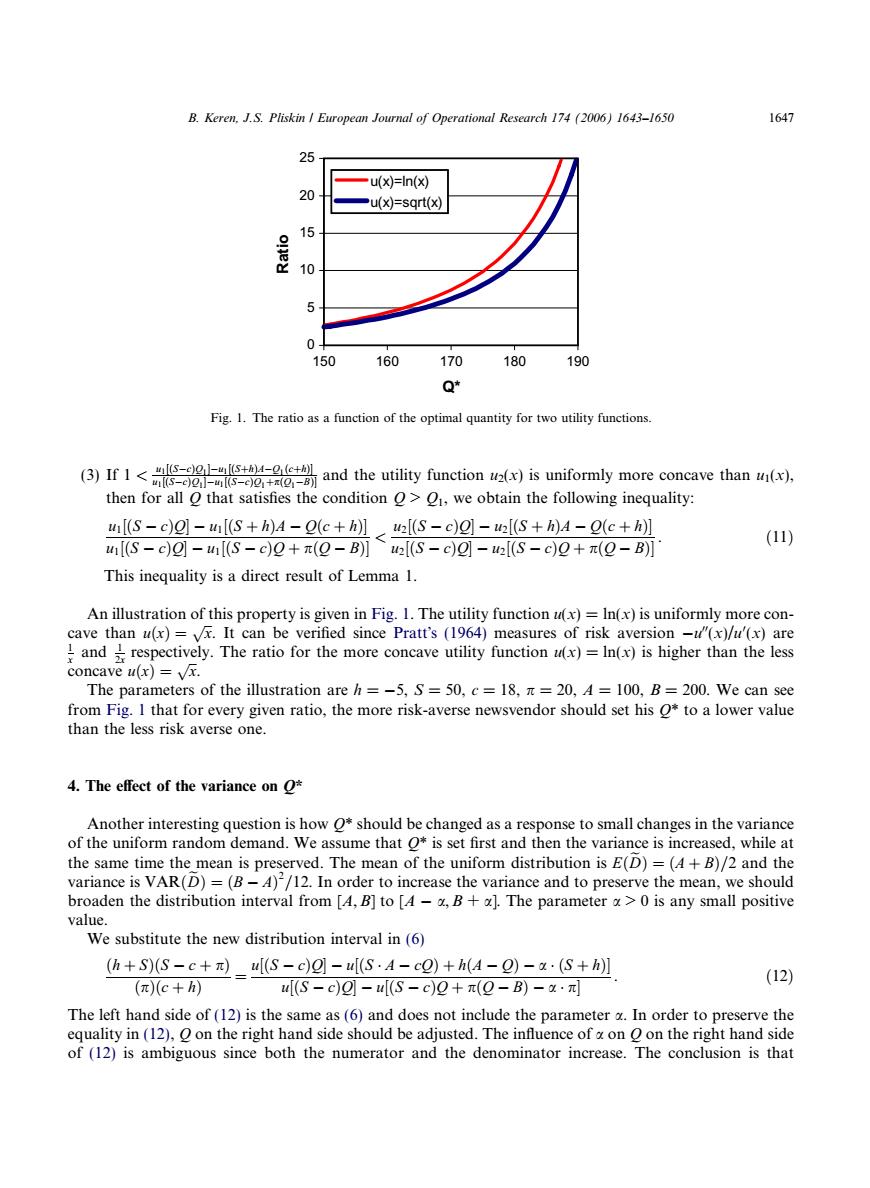
B.Keren.J.S.Pliskin European Journal of Operational Research 174 (2006)1643-1650 1647 25 -u(x)=In(x) 20 -u(x)=sqrt(x) 15 晨 10 04 150 160 170 180 190 Q* Fig.1.The ratio as a function of the optimal quantity for two utility functions. (3)If 1and the utility function (is uniformly more concave than) then for all O that satisfies the condition >1,we obtain the following inequality: ul(s-c)e]-u[(S+h)4-e(c+h]u[(s-c)o]-ua[(S+h)4-(c+h (11) [(S-c)g-[(S-c)0+π(Q-B)】u2l(S-c)g-2[(S-c)2+π(9-B] This inequality is a direct result of Lemma 1. An illustration of this property is given in Fig.1.The utility function u(x)=In(x)is uniformly more con- cave than u(x)=vx.It can be verified since Pratt's (1964)measures of risk aversion -u"(x)/u'(x)are and respectively.The ratio for the more concave utility function u(x)=In(x)is higher than the less concave u(x)=vx. The parameters of the illustration are h=-5,S=50,c=18,n=20,A=100,B=200.We can see from Fig.I that for every given ratio,the more risk-averse newsvendor should set his O*to a lower value than the less risk averse one. 4.The effect of the variance on O* Another interesting question is how o*should be changed as a response to small changes in the variance of the uniform random demand.We assume that O*is set first and then the variance is increased,while at the same time the mean is preserved.The mean of the uniform distribution is E(D)=(A+B)/2 and the variance is VAR(D)=(B-A)/12.In order to increase the variance and to preserve the mean,we should broaden the distribution interval from [A,B]to [A-a,B+a].The parameter >0 is any small positive value. We substitute the new distribution interval in(6) (h+S(S-c+_u(S-cg]-S·A-c2)+h(4-)-·(S+h (12) (π(c+h) [(S-c)g-[(S-c)2+π(Q-B)-x·元 The left hand side of(12)is the same as(6)and does not include the parameter a.In order to preserve the equality in(12),O on the right hand side should be adjusted.The influence of a on O on the right hand side of (12)is ambiguous since both the numerator and the denominator increase.The conclusion is that(3) If 1 < u1½ðScÞQ1u1½ðSþhÞAQ1ðcþhÞ u1½ðScÞQ1u1½ðScÞQ1þpðQ1BÞ and the utility function u2(x) is uniformly more concave than u1(x), then for all Q that satisfies the condition Q > Q1, we obtain the following inequality: u1½ðS cÞQ u1½ðS þ hÞA Qðc þ hÞ u1½ðS cÞQ u1½ðS cÞQ þ pðQ BÞ < u2½ðS cÞQ u2½ðS þ hÞA Qðc þ hÞ u2½ðS cÞQ u2½ðS cÞQ þ pðQ BÞ . ð11Þ This inequality is a direct result of Lemma 1. An illustration of this property is given in Fig. 1. The utility function u(x) = ln(x) is uniformly more con￾cave than uðxÞ ¼ ffiffi x p . It can be verified since Pratts (1964) measures of risk aversion u00(x)/u0 (x) are 1 x and 1 2x respectively. The ratio for the more concave utility function u(x) = ln(x) is higher than the less concave uðxÞ ¼ ffiffi x p . The parameters of the illustration are h = 5, S = 50, c = 18, p = 20, A = 100, B = 200. We can see from Fig. 1 that for every given ratio, the more risk-averse newsvendor should set his Q* to a lower value than the less risk averse one. 4. The effect of the variance on Q* Another interesting question is how Q* should be changed as a response to small changes in the variance of the uniform random demand. We assume that Q* is set first and then the variance is increased, while at the same time the mean is preserved. The mean of the uniform distribution is EðDeÞ¼ðA þ BÞ=2 and the variance is VARðDeÞ¼ðB AÞ 2 =12. In order to increase the variance and to preserve the mean, we should broaden the distribution interval from [A,B] to [A a,B + a]. The parameter a > 0 is any small positive value. We substitute the new distribution interval in (6) ðh þ SÞðS c þ pÞ ðpÞðc þ hÞ ¼ u½ðS cÞQ u½ðS A cQÞ þ hðA QÞ a ðS þ hÞ u½ðS cÞQ u½ðS cÞQ þ pðQ BÞ a p . ð12Þ The left hand side of (12) is the same as (6) and does not include the parameter a. In order to preserve the equality in (12), Q on the right hand side should be adjusted. The influence of a on Q on the right hand side of (12) is ambiguous since both the numerator and the denominator increase. The conclusion is that 0 5 10 15 20 25 150 160 170 180 190 Q* Ratio u(x)=ln(x) u(x)=sqrt(x) Fig. 1. The ratio as a function of the optimal quantity for two utility functions. B. Keren, J.S. Pliskin / European Journal of Operational Research 174 (2006) 1643–1650 1647