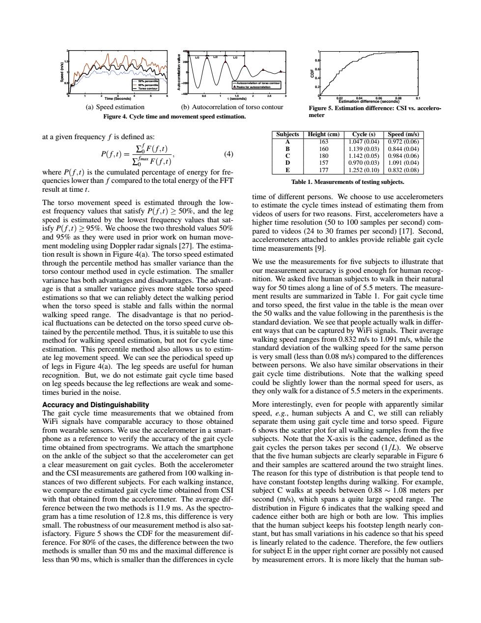
45 t(seconds) 2 25 Estimation difference(seconds) (a)Speed estimation (b)Autocorrelation of torso contour Figure 5.Estimation difference:CSI vs.accelero- Figure 4.Cycle time and movement speed estimation. meter at a given frequency f is defined as: Sūbjects Height(cm) Cycle (s) Speed (m/s) 165 1.0470.04) 0.972(0.06) F(f,) 160 1.139(0.03) 0.844(0.04) P(f,t)= (4) ∑mFf,d) C 180 1.142(0.05) 0.984(0.06) D 157 0.970(0.03) 1.091(0.04) where P(f,t)is the cumulated percentage of energy for fre- E 177 1.252(0.10) 0.832(0.08) quencies lower than f compared to the total energy of the FFT Table 1.Measurements of testing subjects. result at time t. time of different persons.We choose to use accelerometers The torso movement speed is estimated through the low- to estimate the cycle times instead of estimating them from est frequency values that satisfy P(f,t)>50%,and the leg videos of users for two reasons.First,accelerometers have a speed is estimated by the lowest frequency values that sat- higher time resolution(50 to 100 samples per second)com- isfy P(f,t)>95%.We choose the two threshold values 50% pared to videos(24 to 30 frames per second)[17].Second, and 95%as they were used in prior work on human move- accelerometers attached to ankles provide reliable gait cycle ment modeling using Doppler radar signals [27].The estima- time measurements [9]. tion result is shown in Figure 4(a).The torso speed estimated through the percentile method has smaller variance than the We use the measurements for five subjects to illustrate that torso contour method used in cycle estimation.The smaller our measurement accuracy is good enough for human recog- variance has both advantages and disadvantages.The advant- nition.We asked five human subjects to walk in their natural age is that a smaller variance gives more stable torso speed way for 50 times along a line ofof 5.5 meters.The measure- estimations so that we can reliably detect the walking period ment results are summarized in Table 1.For gait cycle time when the torso speed is stable and falls within the normal and torso speed,the first value in the table is the mean over walking speed range.The disadvantage is that no period- the 50 walks and the value following in the parenthesis is the ical fluctuations can be detected on the torso speed curve ob- standard deviation.We see that people actually walk in differ- tained by the percentile method.Thus,it is suitable to use this ent ways that can be captured by WiFi signals.Their average method for walking speed estimation,but not for cycle time walking speed ranges from 0.832 m/s to 1.091 m/s,while the estimation.This percentile method also allows us to estim- standard deviation of the walking speed for the same person ate leg movement speed.We can see the periodical speed up is very small (less than 0.08 m/s)compared to the differences of legs in Figure 4(a).The leg speeds are useful for human between persons.We also have similar observations in their recognition.But,we do not estimate gait cycle time based gait cycle time distributions.Note that the walking speed on leg speeds because the leg reflections are weak and some- could be slightly lower than the normal speed for users,as times buried in the noise. they only walk for a distance of 5.5 meters in the experiments. Accuracy and Distinguishability More interestingly,even for people with apparently similar The gait cycle time measurements that we obtained from speed,e.g.,human subjects A and C,we still can reliably WiFi signals have comparable accuracy to those obtained separate them using gait cycle time and torso speed.Figure from wearable sensors.We use the accelerometer in a smart- 6 shows the scatter plot for all walking samples from the five phone as a reference to verify the accuracy of the gait cycle subjects.Note that the X-axis is the cadence,defined as the time obtained from spectrograms.We attach the smartphone gait cycles the person takes per second (1/L).We observe on the ankle of the subject so that the accelerometer can get that the five human subjects are clearly separable in Figure 6 a clear measurement on gait cycles.Both the accelerometer and their samples are scattered around the two straight lines. and the CSI measurements are gathered from 100 walking in- The reason for this type of distribution is that people tend to stances of two different subjects.For each walking instance, have constant footstep lengths during walking.For example, we compare the estimated gait cycle time obtained from CSI subject C walks at speeds between 0.88~1.08 meters per with that obtained from the accelerometer.The average dif- second(m/s),which spans a quite large speed range.The ference between the two methods is 11.9 ms.As the spectro- distribution in Figure 6 indicates that the walking speed and gram has a time resolution of 12.8 ms,this difference is very cadence either both are high or both are low.This implies small.The robustness of our measurement method is also sat- that the human subject keeps his footstep length nearly con- isfactory.Figure 5 shows the CDF for the measurement dif- stant,but has small variations in his cadence so that his speed ference.For 80%of the cases,the difference between the two is linearly related to the cadence.Therefore,the few outliers methods is smaller than 50 ms and the maximal difference is for subject E in the upper right corner are possibly not caused less than 90 ms,which is smaller than the differences in cycle by measurement errors.It is more likely that the human sub0 1 2 3 4 5 6 0 0.5 1 1.5 2 Time (Seconds) Speed (m/s) 50% percentile 95% percentile Torso contour (a) Speed estimation 0.5 1 1.5 2 2.5 3 −400 −200 0 200 400 τ (seconds) Autocorrelation value Autocorrelation of torso contour Peaks for autocorrelation L/2 L/2 L/2 (b) Autocorrelation of torso contour Figure 4. Cycle time and movement speed estimation. 0 0.02 0.04 0.06 0.08 0.1 0 0.2 0.4 0.6 0.8 1 Estimation difference (seconds) CDF Figure 5. Estimation difference: CSI vs. accelero￾meter at a given frequency f is defined as: P(f,t) = ∑ f 0 F(f,t) ∑ fmax 0 F(f,t) , (4) where P(f,t) is the cumulated percentage of energy for fre￾quencies lower than f compared to the total energy of the FFT result at time t. The torso movement speed is estimated through the low￾est frequency values that satisfy P(f,t) ≥ 50%, and the leg speed is estimated by the lowest frequency values that sat￾isfy P(f,t) ≥ 95%. We choose the two threshold values 50% and 95% as they were used in prior work on human move￾ment modeling using Doppler radar signals [27]. The estima￾tion result is shown in Figure 4(a). The torso speed estimated through the percentile method has smaller variance than the torso contour method used in cycle estimation. The smaller variance has both advantages and disadvantages. The advant￾age is that a smaller variance gives more stable torso speed estimations so that we can reliably detect the walking period when the torso speed is stable and falls within the normal walking speed range. The disadvantage is that no period￾ical fluctuations can be detected on the torso speed curve ob￾tained by the percentile method. Thus, it is suitable to use this method for walking speed estimation, but not for cycle time estimation. This percentile method also allows us to estim￾ate leg movement speed. We can see the periodical speed up of legs in Figure 4(a). The leg speeds are useful for human recognition. But, we do not estimate gait cycle time based on leg speeds because the leg reflections are weak and some￾times buried in the noise. Accuracy and Distinguishability The gait cycle time measurements that we obtained from WiFi signals have comparable accuracy to those obtained from wearable sensors. We use the accelerometer in a smart￾phone as a reference to verify the accuracy of the gait cycle time obtained from spectrograms. We attach the smartphone on the ankle of the subject so that the accelerometer can get a clear measurement on gait cycles. Both the accelerometer and the CSI measurements are gathered from 100 walking in￾stances of two different subjects. For each walking instance, we compare the estimated gait cycle time obtained from CSI with that obtained from the accelerometer. The average dif￾ference between the two methods is 11.9 ms. As the spectro￾gram has a time resolution of 12.8 ms, this difference is very small. The robustness of our measurement method is also sat￾isfactory. Figure 5 shows the CDF for the measurement dif￾ference. For 80% of the cases, the difference between the two methods is smaller than 50 ms and the maximal difference is less than 90 ms, which is smaller than the differences in cycle Subjects Height (cm) Cycle (s) Speed (m/s) A 163 1.047 (0.04) 0.972 (0.06) B 160 1.139 (0.03) 0.844 (0.04) C 180 1.142 (0.05) 0.984 (0.06) D 157 0.970 (0.03) 1.091 (0.04) E 177 1.252 (0.10) 0.832 (0.08) Table 1. Measurements of testing subjects. time of different persons. We choose to use accelerometers to estimate the cycle times instead of estimating them from videos of users for two reasons. First, accelerometers have a higher time resolution (50 to 100 samples per second) com￾pared to videos (24 to 30 frames per second) [17]. Second, accelerometers attached to ankles provide reliable gait cycle time measurements [9]. We use the measurements for five subjects to illustrate that our measurement accuracy is good enough for human recog￾nition. We asked five human subjects to walk in their natural way for 50 times along a line of of 5.5 meters. The measure￾ment results are summarized in Table 1. For gait cycle time and torso speed, the first value in the table is the mean over the 50 walks and the value following in the parenthesis is the standard deviation. We see that people actually walk in differ￾ent ways that can be captured by WiFi signals. Their average walking speed ranges from 0.832 m/s to 1.091 m/s, while the standard deviation of the walking speed for the same person is very small (less than 0.08 m/s) compared to the differences between persons. We also have similar observations in their gait cycle time distributions. Note that the walking speed could be slightly lower than the normal speed for users, as they only walk for a distance of 5.5 meters in the experiments. More interestingly, even for people with apparently similar speed, e.g., human subjects A and C, we still can reliably separate them using gait cycle time and torso speed. Figure 6 shows the scatter plot for all walking samples from the five subjects. Note that the X-axis is the cadence, defined as the gait cycles the person takes per second (1/L). We observe that the five human subjects are clearly separable in Figure 6 and their samples are scattered around the two straight lines. The reason for this type of distribution is that people tend to have constant footstep lengths during walking. For example, subject C walks at speeds between 0.88 ∼ 1.08 meters per second (m/s), which spans a quite large speed range. The distribution in Figure 6 indicates that the walking speed and cadence either both are high or both are low. This implies that the human subject keeps his footstep length nearly con￾stant, but has small variations in his cadence so that his speed is linearly related to the cadence. Therefore, the few outliers for subject E in the upper right corner are possibly not caused by measurement errors. It is more likely that the human sub-