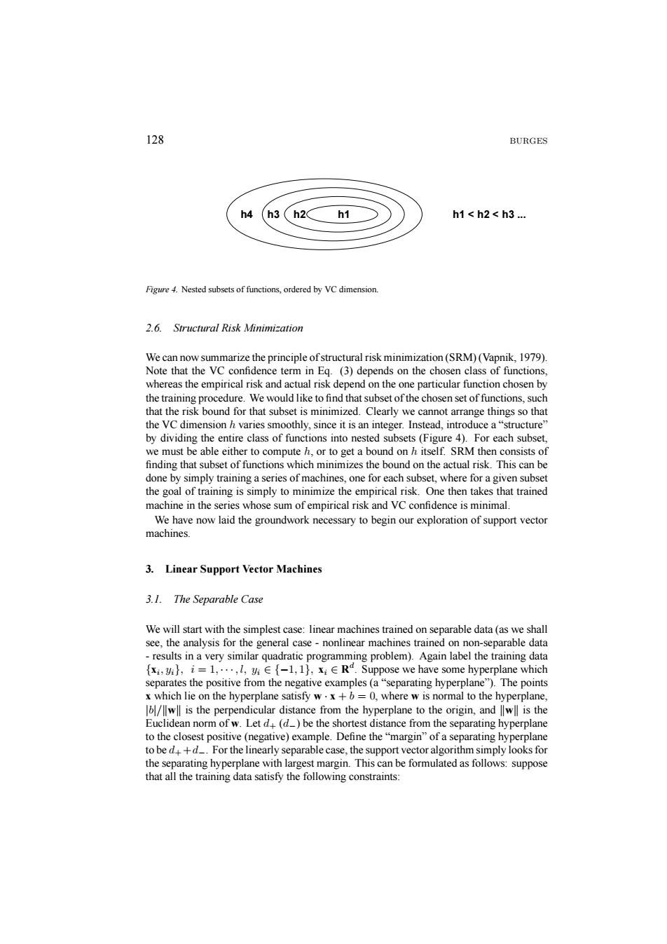
128 BURGES h4 （h3(h2h1 h1<h2<h3 Figure 4.Nested subsets of functions,ordered by VC dimension 2.6.Structural Risk Minimization We can now summarize the principle of structural risk minimization(SRM)(Vapnik,1979). Note that the VC confidence term in Eq.(3)depends on the chosen class of functions, whereas the empirical risk and actual risk depend on the one particular function chosen by the training procedure.We would like to find that subset of the chosen set of functions,such that the risk bound for that subset is minimized.Clearly we cannot arrange things so that the VC dimension h varies smoothly,since it is an integer.Instead,introduce a"structure" by dividing the entire class of functions into nested subsets(Figure 4).For each subset we must be able either to compute h,or to get a bound on h itself.SRM then consists of finding that subset of functions which minimizes the bound on the actual risk.This can be done by simply training a series of machines,one for each subset,where for a given subset the goal of training is simply to minimize the empirical risk.One then takes that trained machine in the series whose sum of empirical risk and VC confidence is minimal. We have now laid the groundwork necessary to begin our exploration of support vector machines. 3.Linear Support Vector Machines 3.1.The Separable Case We will start with the simplest case:linear machines trained on separable data(as we shall see,the analysis for the general case-nonlinear machines trained on non-separable data results in a very similar quadratic programming problem).Again label the training data x,,i=1,...,l,i-1,1),xiE Rd.Suppose we have some hyperplane which separates the positive from the negative examples(a"separating hyperplane").The points x which lie on the hyperplane satisfy w.x+b=0,where w is normal to the hyperplane, wll is the perpendicular distance from the hyperplane to the origin,and lwll is the Euclidean norm of w.Let d(d)be the shortest distance from the separating hyperplane to the closest positive(negative)example.Define the"margin"of a separating hyperplane to be d+d_.For the linearly separable case,the support vector algorithm simply looks for the separating hyperplane with largest margin.This can be formulated as follows:suppose that all the training data satisfy the following constraints:128 BURGES h4 h1 < h2 < h3 ... h3 h2 h1 Figure 4. Nested subsets of functions, ordered by VC dimension. 2.6. Structural Risk Minimization We can now summarize the principle of structural risk minimization (SRM) (Vapnik, 1979). Note that the VC confidence term in Eq. (3) depends on the chosen class of functions, whereas the empirical risk and actual risk depend on the one particular function chosen by the training procedure. We would like to find that subset of the chosen set of functions, such that the risk bound for that subset is minimized. Clearly we cannot arrange things so that the VC dimension h varies smoothly, since it is an integer. Instead, introduce a “structure” by dividing the entire class of functions into nested subsets (Figure 4). For each subset, we must be able either to compute h, or to get a bound on h itself. SRM then consists of finding that subset of functions which minimizes the bound on the actual risk. This can be done by simply training a series of machines, one for each subset, where for a given subset the goal of training is simply to minimize the empirical risk. One then takes that trained machine in the series whose sum of empirical risk and VC confidence is minimal. We have now laid the groundwork necessary to begin our exploration of support vector machines. 3. Linear Support Vector Machines 3.1. The Separable Case We will start with the simplest case: linear machines trained on separable data (as we shall see, the analysis for the general case - nonlinear machines trained on non-separable data - results in a very similar quadratic programming problem). Again label the training data {xi, yi}, i = 1, ··· ,l, yi ∈ {−1, 1}, xi ∈ Rd. Suppose we have some hyperplane which separates the positive from the negative examples (a “separating hyperplane”). The points x which lie on the hyperplane satisfy w · x + b = 0, where w is normal to the hyperplane, |b|/kwk is the perpendicular distance from the hyperplane to the origin, and kwk is the Euclidean norm of w. Let d+ (d−) be the shortest distance from the separating hyperplane to the closest positive (negative) example. Define the “margin” of a separating hyperplane to be d+ +d−. For the linearly separable case, the support vector algorithm simply looks for the separating hyperplane with largest margin. This can be formulated as follows: suppose that all the training data satisfy the following constraints: