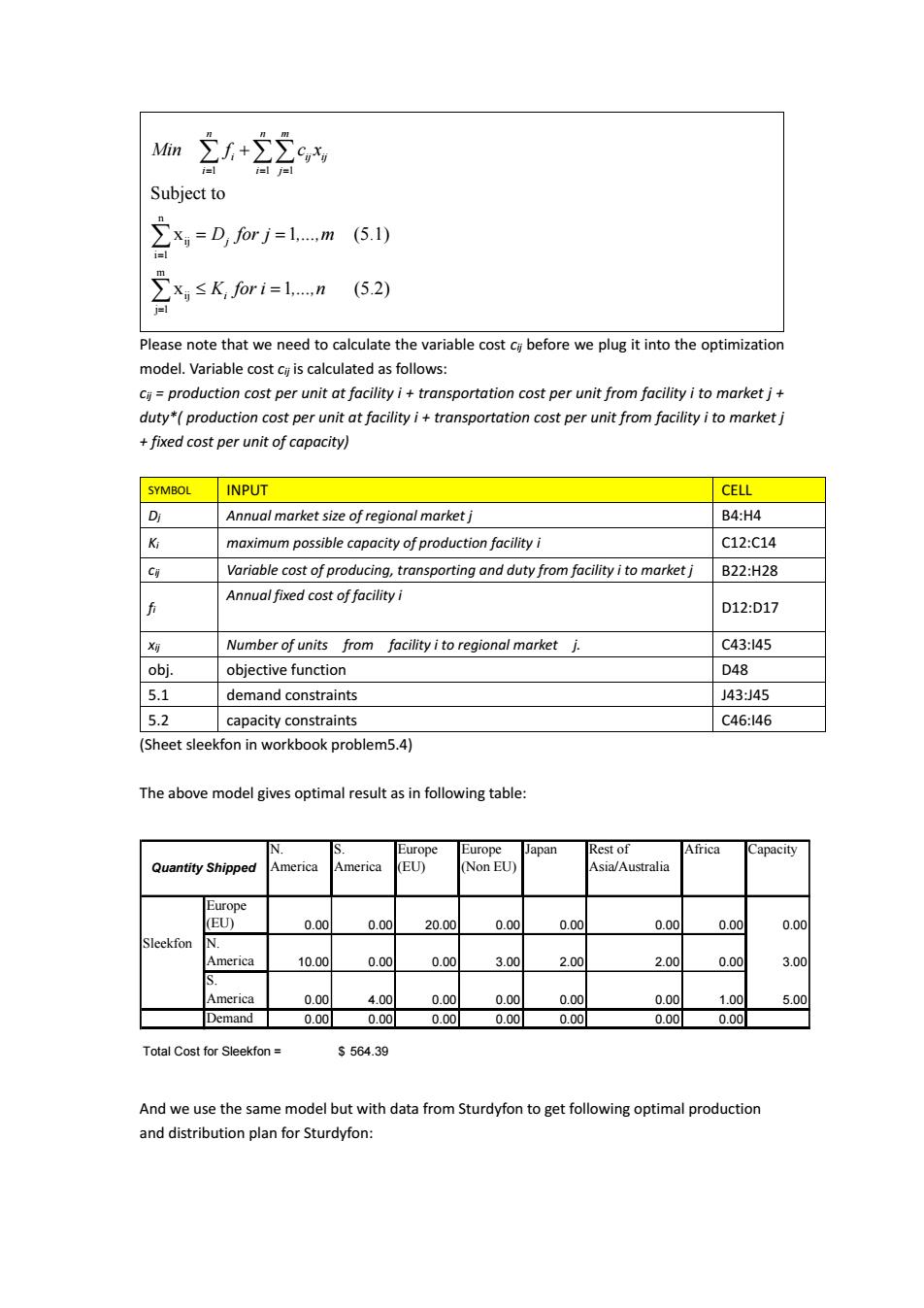
Min 21+22 i=l i=l i=l Subject to x=D,forj =1....m (5.1) xk,for 1=1.m (5.2) Please note that we need to calculate the variable cost cy before we plug it into the optimization model.Variable cost cyj is calculated as follows: cj=production cost per unit at facility i transportation cost per unit from facility i to market j+ duty*(production cost per unit at facility i+transportation cost per unit from facility i to market j fixed cost per unit of capacity) SYMBOL INPUT CELL D Annual market size of regional market j B4:H4 K maximum possible capacity of production facility i C12:C14 Ci Variable cost of producing,transporting and duty from facility i to market j B22:H28 Annual fixed cost of facility i 币 D12:D17 Number of units from facility i to regional market j. C43:l45 obj. objective function D48 5.1 demand constraints J43J45 5.2 capacity constraints C46:l46 (Sheet sleekfon in workbook problem5.4) The above model gives optimal result as in following table: N. Europe Europe Japan Rest of Africa Capacity Quantity Shipped America America (EU) (Non EU) Asia/Australia Europe (EU) 0.00 0.00 20.00 0.00 0.00 0.00 0.00 0.00 Sleekfon America 10.00 0.00 0.00 3.00 2.00 2.00 0.00 3.00 不 America 0.00 4.00 0.00 0.00 0.00 0.00 1.00 5.00 Demand 0.00 0.00 0.00 0.00 0.00 0.00 0.00 Total Cost for Sleekfon S564.39 And we use the same model but with data from Sturdyfon to get following optimal production and distribution plan for Sturdyfon:1 1 1 n ij i 1 m ij j 1 Subject to x 1 (5.1) x 1 (5.2) n n m i ij ij i i j j i Min f c x D for j ,...,m K for i ,...,n               Please note that we need to calculate the variable cost cij before we plug it into the optimization model. Variable cost cij is calculated as follows: cij = production cost per unit at facility i + transportation cost per unit from facility i to market j + duty*( production cost per unit at facility i + transportation cost per unit from facility i to market j + fixed cost per unit of capacity) SYMBOL INPUT CELL Dj Annual market size of regional market j B4:H4 Ki maximum possible capacity of production facility i C12:C14 cij Variable cost of producing, transporting and duty from facility i to market j B22:H28 fi Annual fixed cost of facility i D12:D17 xij Number of units from facility i to regional market j. C43:I45 obj. objective function D48 5.1 demand constraints J43:J45 5.2 capacity constraints C46:I46 (Sheet sleekfon in workbook problem5.4) The above model gives optimal result as in following table: And we use the same model but with data from Sturdyfon to get following optimal production and distribution plan for Sturdyfon: N. America S. America Europe (EU) Europe (Non EU) Japan Rest of Asia/Australia Africa Capacity Europe (EU) 0.00 0.00 20.00 0.00 0.00 0.00 0.00 0.00 Sleekfon N. America 10.00 0.00 0.00 3.00 2.00 2.00 0.00 3.00 S. America 0.00 4.00 0.00 0.00 0.00 0.00 1.00 5.00 Demand 0.00 0.00 0.00 0.00 0.00 0.00 0.00 Total Cost for Sleekfon = $ 564.39 Quantity Shipped