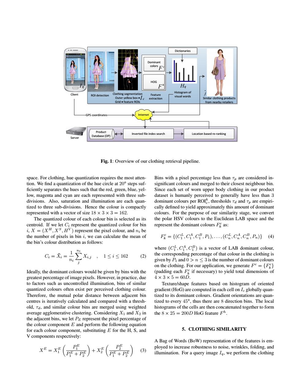
Dictionaries Dominant HOG Ha Client ROl detection Clothing segmentation Histogram of Feature Outer vellow box visual words extraction Similar clothing products Grid feature ROls from nearby retailers GPS coordinates- Product Inverted file index search Location based re-ranking Server Database(DP) Fig.1:Overview of our clothing retrieval pipeline. space.For clothing,hue quantization requires the most atten- Bins with a pixel percentage less than Tp are considered in- tion.We find a quantization of the hue circle at 20 steps suf- significant colours and merged to their closest neighbour bin. ficiently separates the hues such that the red,green,blue,yel- Since each set of worn upper body clothing in our product low,magenta and cyan are each represented with three sub- dataset is humanly perceived to generally have less than 3 divisions.Also,saturation and illumination are each quan- dominant colours per ROI,thresholds Ta and Tp are empiri- tized to three sub-divisions.Hence the colour is compactly cally defined to yield approximately this amount of dominant represented with a vector of size 18×3×3=l62. colours.For the purpose of our similarity stage,we convert The quantized colour of each colour bin is selected as its the polar HSV colours to the Euclidean LAB space and the centroid.If we let Ci represent the quantized colour for bin represent the dominant colours Fe as: i,X=(,XS,HV)represent the pixel colour,and ni be the number of pixels in bin i.we can calculate the mean of F={(CL,CA,CB,P),...(CL CA,CB,Pn)(4) the bin's colour distribution as follows where(CL,CA,Cf)is a vector of LAB dominant colour, 1≤i≤162 (2) the corresponding percentage of that colour in the clothing is ni given by Pi and 0>n<3 is the number of dominant colours on the clothing.For our application,we generate Fe=[Fe} Ideally,the dominant colours would be given by bins with the (padding each Fe if necessary)to yield total dimensions of greatest percentage of image pixels.However,in practice,due 4×3×5=60D. to factors such as uncontrolled illumination,bins of similar Texture/shape features based on histogram of oriented quantized colours often exist per perceived clothing colour. gradient(HoG)are computed in each cell on Ie globally quan- Therefore,the mutual polar distance between adjacent bin tized to its dominant colours.Gradient orientations are quan- centres is iteratively calculated and compared with a thresh- tized to every 45,thus there are 8 direction bins.The local old,Td,and similar colour bins are merged using weighted histograms of the cells are then concatenated together to form average agglomerative clustering.Considering Xi and X2 in the 8 x 25 200D HoG feature Fh. the adjacent bins,we let Pe represent the pixel percentage of the colour component E and perform the following equation for each colour component,substituting E for the H.S,and 5.CLOTHING SIMILARITY V components respectively: A Bag of Words(Bow)representation of the features is em- （P+PE+x ployed to increase robustness to noise,wrinkles,folding,and (3) illumination.For a query image Ig,we perform the clothingROI detection Clothing segmentation Outer yellow box = Grid = feature ROIs Histogram of visual words Dictionaries Feature extraction Similar clothing products from nearby retailers Dominant colors HOG Client Server Internet Product Database (DP) Inverted file index search Hq j ˆ I c c F h F GPS coordinates Location based re-ranking I q Fig. 1: Overview of our clothing retrieval pipeline. space. For clothing, hue quantization requires the most atten￾tion. We find a quantization of the hue circle at 20◦ steps suf- ficiently separates the hues such that the red, green, blue, yel￾low, magenta and cyan are each represented with three sub￾divisions. Also, saturation and illumination are each quan￾tized to three sub-divisions. Hence the colour is compactly represented with a vector of size 18 × 3 × 3 = 162. The quantized colour of each colour bin is selected as its centroid. If we let Ci represent the quantized colour for bin i, X = (XH, XS, HV ) represent the pixel colour, and ni be the number of pixels in bin i, we can calculate the mean of the bin’s colour distribution as follows: Ci = X¯ i = 1 ni Xni j Xi,j , 1 ≤ i ≤ 162 (2) Ideally, the dominant colours would be given by bins with the greatest percentage of image pixels. However, in practice, due to factors such as uncontrolled illumination, bins of similar quantized colours often exist per perceived clothing colour. Therefore, the mutual polar distance between adjacent bin centres is iteratively calculated and compared with a thresh￾old, τd, and similar colour bins are merged using weighted average agglomerative clustering. Considering X1 and X2 in the adjacent bins, we let PE represent the pixel percentage of the colour component E and perform the following equation for each colour component, substituting E for the H, S, and V components respectively: XE = XE 1  P E 1 P E 1 + P E 2  + XE 2  P E 2 P E 1 + P E 2  (3) Bins with a pixel percentage less than τp are considered in￾significant colours and merged to their closest neighbour bin. Since each set of worn upper body clothing in our product dataset is humanly perceived to generally have less than 3 dominant colours per ROIk c , thresholds τd and τp are empiri￾cally defined to yield approximately this amount of dominant colours. For the purpose of our similarity stage, we convert the polar HSV colours to the Euclidean LAB space and the represent the dominant colours F c k as: F c k = {(C L 1 , CA 1 , CB 1 , P1), . . . ,(C L n , CA n , CB n , Pn)} (4) where (C L 1 , CA 1 , CB 1 ) is a vector of LAB dominant colour, the corresponding percentage of that colour in the clothing is given by P1 and 0 > n ≤ 3 is the number of dominant colours on the clothing. For our application, we generate F c = {F c k } (padding each F c k if necessary) to yield total dimensions of 4 × 3 × 5 = 60D. Texture/shape features based on histogram of oriented gradient (HoG) are computed in each cell on Ic globally quan￾tized to its dominant colours. Gradient orientations are quan￾tized to every 45◦ , thus there are 8 direction bins. The local histograms of the cells are then concatenated together to form the 8 × 25 = 200D HoG feature F h . 5. CLOTHING SIMILARITY A Bag of Words (BoW) representation of the features is em￾ployed to increase robustness to noise, wrinkles, folding, and illumination. For a query image Iq, we perform the clothing