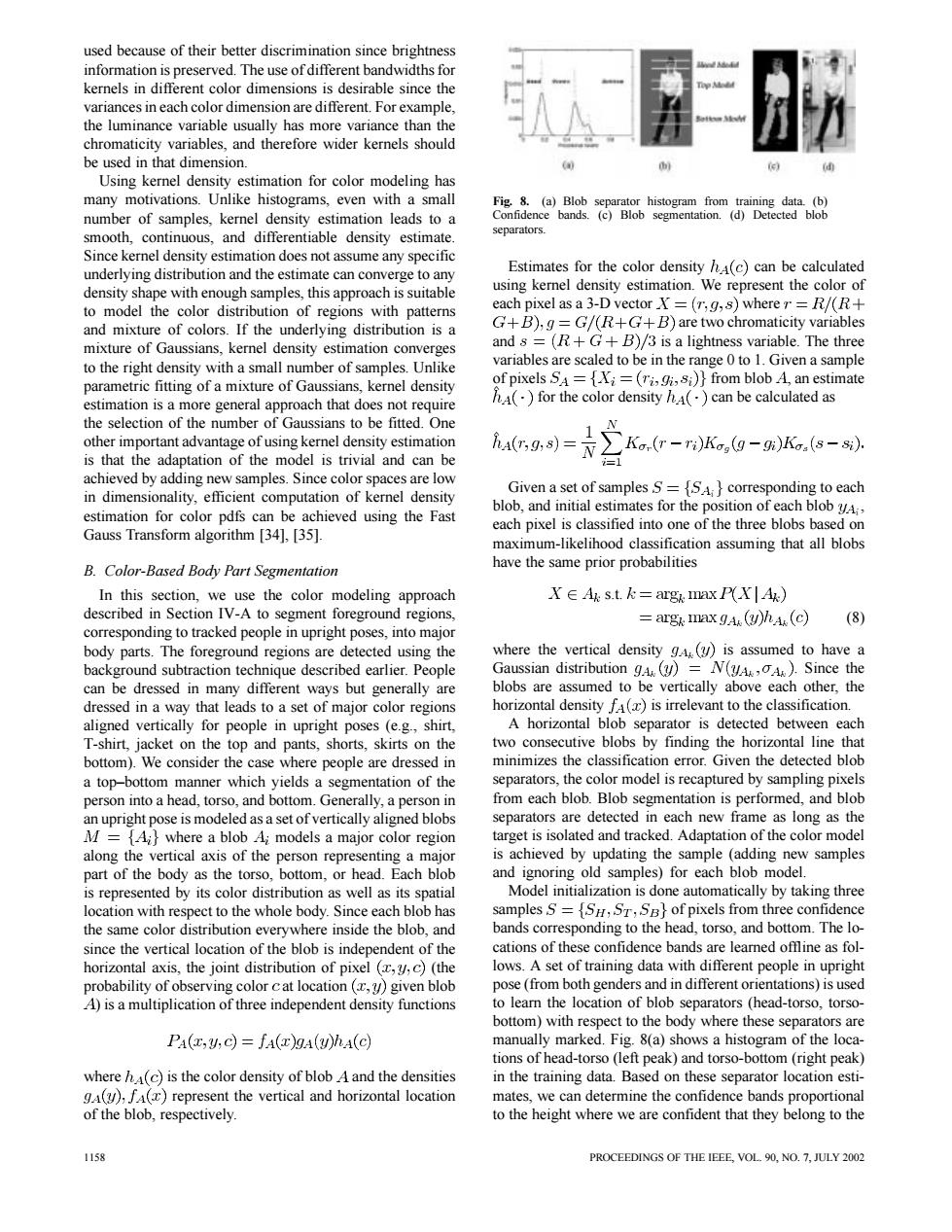
used because of their better discrimination since brightness information is preserved.The use of different bandwidths for kernels in different color dimensions is desirable since the variances in each color dimension are different.For example. the luminance variable usually has more variance than the chromaticity variables,and therefore wider kernels should be used in that dimension. Using kernel density estimation for color modeling has many motivations.Unlike histograms,even with a small Fig.8.(a)Blob separator histogram from training data.(b) number of samples,kernel density estimation leads to a Confidence bands.(c)Blob segmentation.(d)Detected blob smooth,continuous,and differentiable density estimate. separators. Since kernel density estimation does not assume any specific underlying distribution and the estimate can converge to any Estimates for the color density hA(c)can be calculated density shape with enough samples,this approach is suitable using kernel density estimation.We represent the color of to model the color distribution of regions with patterns each pixel as a 3-D vectorX=(r,g,s)wherer=R/(R+ and mixture of colors.If the underlying distribution is a G+B),g=G/(R+G+B)are two chromaticity variables mixture of Gaussians,kernel density estimation converges and s=(R+G+B)/3 is a lightness variable.The three to the right density with a small number of samples.Unlike variables are scaled to be in the range 0 to 1.Given a sample parametric fitting of a mixture of Gaussians,kernel density of pixels SA=i=(ri,gi,si)}from blob A,an estimate estimation is a more general approach that does not require A()for the color density hA()can be calculated as the selection of the number of Gaussians to be fitted.One other important advantage of using kernel density estimation Kar(T-Ti)Kog(g-gi)Koa(s-si). is that the adaptation of the model is trivial and can be achieved by adding new samples.Since color spaces are low in dimensionality,efficient computation of kernel density Given a set of samples S=SA corresponding to each blob,and initial estimates for the position of each blob yA, estimation for color pdfs can be achieved using the Fast each pixel is classified into one of the three blobs based on Gauss Transform algorithm [34],[35]. maximum-likelihood classification assuming that all blobs B.Color-Based Body Part Segmentation have the same prior probabilities In this section,we use the color modeling approach X∈A4ks.tk=aug脉nax P(X|Ak) described in Section IV-A to segment foreground regions, =ag脉nax gA(y)hA(C) (8) corresponding to tracked people in upright poses,into major body parts.The foreground regions are detected using the where the vertical density gAr(y)is assumed to have a background subtraction technique described earlier.People Gaussian distribution gA()=N(yA,A )Since the can be dressed in many different ways but generally are blobs are assumed to be vertically above each other,the dressed in a way that leads to a set of major color regions horizontal density fA()is irrelevant to the classification. aligned vertically for people in upright poses (e.g.,shirt, A horizontal blob separator is detected between each T-shirt,jacket on the top and pants,shorts,skirts on the two consecutive blobs by finding the horizontal line that bottom).We consider the case where people are dressed in minimizes the classification error.Given the detected blob a top-bottom manner which yields a segmentation of the separators,the color model is recaptured by sampling pixels person into a head,torso,and bottom.Generally,a person in from each blob.Blob segmentation is performed,and blob an upright pose is modeled as a set of vertically aligned blobs separators are detected in each new frame as long as the M=Ai}where a blob A;models a major color region target is isolated and tracked.Adaptation of the color model along the vertical axis of the person representing a major is achieved by updating the sample (adding new samples part of the body as the torso,bottom,or head.Each blob and ignoring old samples)for each blob model. is represented by its color distribution as well as its spatial Model initialization is done automatically by taking three location with respect to the whole body.Since each blob has samples S={SH,ST,SB}of pixels from three confidence the same color distribution everywhere inside the blob,and bands corresponding to the head,torso,and bottom.The lo- since the vertical location of the blob is independent of the cations of these confidence bands are learned offline as fol- horizontal axis,the joint distribution of pixel (,y,c)(the lows.A set of training data with different people in upright probability of observing color cat location(,y)given blob pose (from both genders and in different orientations)is used A)is a multiplication of three independent density functions to learn the location of blob separators (head-torso,torso- bottom)with respect to the body where these separators are PA(T,U,C)=fA(T)gA(U)hA(C) manually marked.Fig.8(a)shows a histogram of the loca- tions of head-torso (left peak)and torso-bottom (right peak) where hA(c)is the color density of blob Aand the densities in the training data.Based on these separator location esti- gA(y),fA()represent the vertical and horizontal location mates,we can determine the confidence bands proportional of the blob,respectively. to the height where we are confident that they belong to the 1158 PROCEEDINGS OF THE IEEE,VOL.90,NO.7,JULY 2002used because of their better discrimination since brightness information is preserved. The use of different bandwidths for kernels in different color dimensions is desirable since the variances in each color dimension are different. For example, the luminance variable usually has more variance than the chromaticity variables, and therefore wider kernels should be used in that dimension. Using kernel density estimation for color modeling has many motivations. Unlike histograms, even with a small number of samples, kernel density estimation leads to a smooth, continuous, and differentiable density estimate. Since kernel density estimation does not assume any specific underlying distribution and the estimate can converge to any density shape with enough samples, this approach is suitable to model the color distribution of regions with patterns and mixture of colors. If the underlying distribution is a mixture of Gaussians, kernel density estimation converges to the right density with a small number of samples. Unlike parametric fitting of a mixture of Gaussians, kernel density estimation is a more general approach that does not require the selection of the number of Gaussians to be fitted. One other important advantage of using kernel density estimation is that the adaptation of the model is trivial and can be achieved by adding new samples. Since color spaces are low in dimensionality, efficient computation of kernel density estimation for color pdfs can be achieved using the Fast Gauss Transform algorithm [34], [35]. B. Color-Based Body Part Segmentation In this section, we use the color modeling approach described in Section IV-A to segment foreground regions, corresponding to tracked people in upright poses, into major body parts. The foreground regions are detected using the background subtraction technique described earlier. People can be dressed in many different ways but generally are dressed in a way that leads to a set of major color regions aligned vertically for people in upright poses (e.g., shirt, T-shirt, jacket on the top and pants, shorts, skirts on the bottom). We consider the case where people are dressed in a top–bottom manner which yields a segmentation of the person into a head, torso, and bottom. Generally, a person in an upright pose is modeled as a set of vertically aligned blobs where a blob models a major color region along the vertical axis of the person representing a major part of the body as the torso, bottom, or head. Each blob is represented by its color distribution as well as its spatial location with respect to the whole body. Since each blob has the same color distribution everywhere inside the blob, and since the vertical location of the blob is independent of the horizontal axis, the joint distribution of pixel (the probability of observing color at location given blob ) is a multiplication of three independent density functions where is the color density of blob and the densities represent the vertical and horizontal location of the blob, respectively. Fig. 8. (a) Blob separator histogram from training data. (b) Confidence bands. (c) Blob segmentation. (d) Detected blob separators. Estimates for the color density can be calculated using kernel density estimation. We represent the color of each pixel as a 3-D vector where are two chromaticity variables and is a lightness variable. The three variables are scaled to be in the range 0 to 1. Given a sample of pixels from blob , an estimate for the color density can be calculated as Given a set of samples corresponding to each blob, and initial estimates for the position of each blob , each pixel is classified into one of the three blobs based on maximum-likelihood classification assuming that all blobs have the same prior probabilities s.t. (8) where the vertical density is assumed to have a Gaussian distribution . Since the blobs are assumed to be vertically above each other, the horizontal density is irrelevant to the classification. A horizontal blob separator is detected between each two consecutive blobs by finding the horizontal line that minimizes the classification error. Given the detected blob separators, the color model is recaptured by sampling pixels from each blob. Blob segmentation is performed, and blob separators are detected in each new frame as long as the target is isolated and tracked. Adaptation of the color model is achieved by updating the sample (adding new samples and ignoring old samples) for each blob model. Model initialization is done automatically by taking three samples of pixels from three confidence bands corresponding to the head, torso, and bottom. The lo￾cations of these confidence bands are learned offline as fol￾lows. A set of training data with different people in upright pose (from both genders and in different orientations) is used to learn the location of blob separators (head-torso, torso￾bottom) with respect to the body where these separators are manually marked. Fig. 8(a) shows a histogram of the loca￾tions of head-torso (left peak) and torso-bottom (right peak) in the training data. Based on these separator location esti￾mates, we can determine the confidence bands proportional to the height where we are confident that they belong to the 1158 PROCEEDINGS OF THE IEEE, VOL. 90, NO. 7, JULY 2002