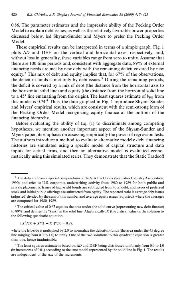
420 R.S.Chirinko.A.R.Singha Journal of Financial Economics 58 (2000)417-425 0.86.The parameter estimates and the impressive ability of the Pecking Order Model to explain debt issues,as well as the relatively favorable power properties discussed below,led Shyam-Sunder and Myers to prefer the Pecking Order Model. These empirical results can be interpreted in terms of a simple graph.Fig.1 plots AD and DEF on the vertical and horizontal axes,respectively,and, without loss in generality,these variables range from zero to unity.Assume that there are 100 time periods and,consistent with aggregate data,89%of external financing needs are met by new debt with the remaining deficit covered by new equity.2 This mix of debt and equity implies that,for 67%of the observations, the deficit-in-funds is met only by debt issues.3 During the remaining periods, the deficit is covered by a mix of debt (the distance from the horizontal axis to the horizontal solid line)and equity(the distance from the horizontal solid line to a 45 line emanating from the origin).The least squares estimate of bpo from this model is 0.74.4 Thus,the data graphed in Fig.1 reproduce Shyam-Sunder and Myers'empirical results,which are consistent with the semi-strong form of the Pecking Order Model recognizing equity finance at the bottom of the financing hierarchy. Before evaluating the ability of Eq.(1)to discriminate among competing hypotheses,we mention another important aspect of the Shyam-Sunder and Myers paper,its emphasis on assessing empirically the power of regression tests. The authors introduce a method to evaluate alternative models:debt financing histories are simulated using a specific model of capital structure and data inputs for actual firms,and then an alternative model is evaluated econo- metrically using this simulated series.They demonstrate that the Static Tradeoff 2The data are from a special compendium of the SIA Fact Book(Securities Industry Association, 1990),and refer to U.S.corporate underwriting activity from 1980 to 1989 for both public and private placements.Issues of high-yield bonds are subtracted from total debt,and issues of preferred stock and initial public offerings are subtracted from equity.The reported ratio is average debt issues (adjusted)divided by the sum of this number and average equity issues(adjusted),where the averages are computed for 1980-1989. 3 The critical value of 0.67 equates the area under the solid curve(representing new debt finance) to 89%,and defines the "kink"in the solid line.Algebraically,X (the critical value)is the solution to the following quadratic equation: [X220+X*(1-X]2.0=0.89, where the left-side is multiplied by 2.0 to normalize the deficit-in-funds(the area under the 45 degree line ranging from 0.0 to 1.0)to unity.One of the two solutions to this quadratic equation is greater than one,hence inadmissible. 4The least squares estimate is based on AD and DEF being distributed uniformly from 0.0 to 1.0 (in increments of 0.01)according to the true model represented by the solid line in Fig.1.The results are independent of the size of the increments.2The data are from a special compendium of the SIA Fact Book (Securities Industry Association, 1990), and refer to U.S. corporate underwriting activity from 1980 to 1989 for both public and private placements. Issues of high-yield bonds are subtracted from total debt, and issues of preferred stock and initial public o!erings are subtracted from equity. The reported ratio is average debt issues (adjusted) divided by the sum of this number and average equity issues (adjusted), where the averages are computed for 1980}1989. 3The critical value of 0.67 equates the area under the solid curve (representing new debt "nance) to 89%, and de"nes the `kinka in the solid line. Algebraically, X (the critical value) is the solution to the following quadratic equation: [X2/2.0#XH(1!X)]H2.0"0.89, where the left-side is multiplied by 2.0 to normalize the de"cit-in-funds (the area under the 45 degree line ranging from 0.0 to 1.0) to unity. One of the two solutions to this quadratic equation is greater than one, hence inadmissible. 4The least squares estimate is based on *D and DEF being distributed uniformly from 0.0 to 1.0 (in increments of 0.01) according to the true model represented by the solid line in Fig. 1. The results are independent of the size of the increments. 0.86. The parameter estimates and the impressive ability of the Pecking Order Model to explain debt issues, as well as the relatively favorable power properties discussed below, led Shyam-Sunder and Myers to prefer the Pecking Order Model. These empirical results can be interpreted in terms of a simple graph. Fig. 1 plots *D and DEF on the vertical and horizontal axes, respectively, and, without loss in generality, these variables range from zero to unity. Assume that there are 100 time periods and, consistent with aggregate data, 89% of external "nancing needs are met by new debt with the remaining de"cit covered by new equity.2 This mix of debt and equity implies that, for 67% of the observations, the de"cit-in-funds is met only by debt issues.3 During the remaining periods, the de"cit is covered by a mix of debt (the distance from the horizontal axis to the horizontal solid line) and equity (the distance from the horizontal solid line to a 453 line emanating from the origin). The least squares estimate of b PO from this model is 0.74.4 Thus, the data graphed in Fig. 1 reproduce Shyam-Sunder and Myers' empirical results, which are consistent with the semi-strong form of the Pecking Order Model recognizing equity "nance at the bottom of the "nancing hierarchy. Before evaluating the ability of Eq. (1) to discriminate among competing hypotheses, we mention another important aspect of the Shyam-Sunder and Myers paper, its emphasis on assessing empirically the power of regression tests. The authors introduce a method to evaluate alternative models: debt "nancing histories are simulated using a speci"c model of capital structure and data inputs for actual "rms, and then an alternative model is evaluated econo￾metrically using this simulated series. They demonstrate that the Static Tradeo! 420 R.S. Chirinko, A.R. Singha / Journal of Financial Economics 58 (2000) 417}425