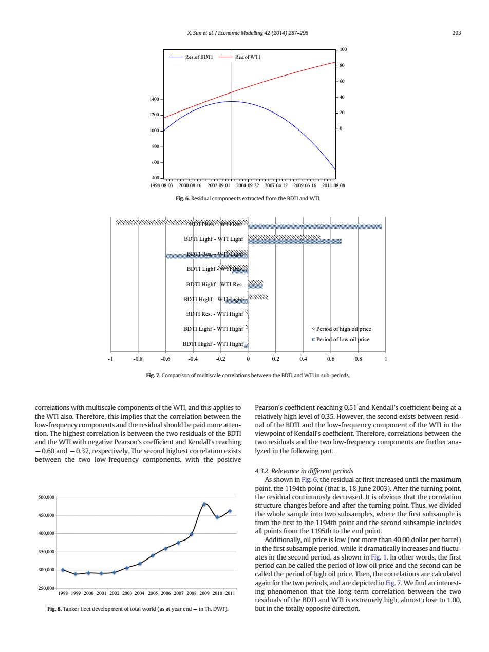
X.Sun et al Economic Modelling 42 (2014)287-295 293 100 Res.of BDTI Res.ofWTI 60 1400 40 1200, 1000. 0 800. 600 400- TTT7 TTTTTTTTTT 1998.08.032000.08.162002.09.012004.09.222007.04.122009.06.162011.08.08 Fig.6.Residual components extracted from the BDTI and WTI D BDTI Lighf-WTI Lighf BDTIRes-WTELRSAY BDTI Lighf BDTI Highf-WTI Res. BDTI Highf-WTILighf P BDTI Res.-WTI Highf BDTI Lighf-WTI Highf Period of high oil price Period of low oil price BDTI Highf-WTI Highf -0.8 -0.6 0.4 -0.2 0 02 0.4 0.6 0.8 Fig.7.Comparison of multiscale correlations between the BDTI and WTI in sub-periods. correlations with multiscale components of the WTI,and this applies to Pearson's coefficient reaching 0.51 and Kendall's coefficient being at a the WTl also.Therefore,this implies that the correlation between the relatively high level of 0.35.However,the second exists between resid- low-frequency components and the residual should be paid more atten- ual of the BDTI and the low-frequency component of the WTI in the tion.The highest correlation is between the two residuals of the BDTI viewpoint of Kendall's coefficient.Therefore,correlations between the and the WTI with negative Pearson's coefficient and Kendall's reaching two residuals and the two low-frequency components are further ana- -0.60 and-0.37,respectively.The second highest correlation exists lyzed in the following part. between the two low-frequency components,with the positive 4.3.2.Relevance in different periods As shown in Fig.6,the residual at first increased until the maximum point,the 1194th point (that is,18 June 2003).After the turning point, s00,000 the residual continuously decreased.It is obvious that the correlation structure changes before and after the turning point.Thus,we divided 450.000 the whole sample into two subsamples,where the first subsample is from the first to the 1194th point and the second subsample includes 400.000 all points from the 1195th to the end point. Additionally,oil price is low(not more than 40.00 dollar per barrel) 350.000 in the first subsample period,while it dramatically increases and fluctu- ates in the second period,as shown in Fig.1.In other words,the first period can be called the period of low oil price and the second can be 300.000 called the period of high oil price.Then,the correlations are calculated again for the two periods,and are depicted in Fig.7.We find an interest- 250,000- 19981999200020012002200320042005200620072008200920102011 ing phenomenon that the long-term correlation between the two residuals of the BDTI and WTI is extremely high,almost close to 1.00, Fig.8.Tanker fleet development of total world (as at year end-in Th.DWT). but in the totally opposite direction.correlations with multiscale components of the WTI, and this applies to the WTI also. Therefore, this implies that the correlation between the low-frequency components and the residual should be paid more atten￾tion. The highest correlation is between the two residuals of the BDTI and the WTI with negative Pearson's coefficient and Kendall's reaching −0.60 and −0.37, respectively. The second highest correlation exists between the two low-frequency components, with the positive Pearson's coefficient reaching 0.51 and Kendall's coefficient being at a relatively high level of 0.35. However, the second exists between resid￾ual of the BDTI and the low-frequency component of the WTI in the viewpoint of Kendall's coefficient. Therefore, correlations between the two residuals and the two low-frequency components are further ana￾lyzed in the following part. 4.3.2. Relevance in different periods As shown in Fig. 6, the residual at first increased until the maximum point, the 1194th point (that is, 18 June 2003). After the turning point, the residual continuously decreased. It is obvious that the correlation structure changes before and after the turning point. Thus, we divided the whole sample into two subsamples, where the first subsample is from the first to the 1194th point and the second subsample includes all points from the 1195th to the end point. Additionally, oil price is low (not more than 40.00 dollar per barrel) in the first subsample period, while it dramatically increases and fluctu￾ates in the second period, as shown in Fig. 1. In other words, the first period can be called the period of low oil price and the second can be called the period of high oil price. Then, the correlations are calculated again for the two periods, and are depicted in Fig. 7. We find an interest￾ing phenomenon that the long-term correlation between the two residuals of the BDTI and WTI is extremely high, almost close to 1.00, but in the totally opposite direction. 400 600 800 1000 1200 1400 0 20 40 60 80 100 Res.of BDTI Res.of WTI 1998.08.03 2000.08.16 2002.09.01 2004.09.22 2007.04.12 2009.06.16 2011.08.08 Fig. 6. Residual components extracted from the BDTI and WTI. -1 -0.8 -0.6 -0.4 -0.2 0 0.2 0.4 0.6 0.8 1 BDTI Highf - WTI Highf BDTI Lighf - WTI Highf BDTI Res. - WTI Highf BDTI Highf - WTI Lighf BDTI Highf - WTI Res. BDTI Lighf - WTI Res. BDTI Res. - WTI Lighf BDTI Lighf - WTI Lighf BDTI Res. - WTI Res. Period of high oil price Period of low oil price Fig. 7. Comparison of multiscale correlations between the BDTI and WTI in sub-periods. 250,000 300,000 350,000 400,000 450,000 500,000 1998 1999 2000 2001 2002 2003 2004 2005 2006 2007 2008 2009 2010 2011 Fig. 8. Tanker fleet development of total world (as at year end — in Th. DWT). X. Sun et al. / Economic Modelling 42 (2014) 287–295 293