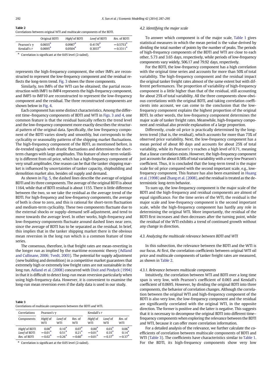
292 X.Sun et aL Economic Modelling 42 (2014)287-295 Table 2 4.2.Identifying the major scale Correlations between original WTI and multiscale components of the BDTI. Original BDTI Highf of BDTI Lowf of BDTI Res.of BDTI To answer which component is of the major scale,Table 1 gives Pearson's v 0.0655* 0.0987* 0.4170 -0.5753* statistical measures in which the mean period is the value derived by Kendall'sT 0.0695* 0.0504 0.3037* -0.3311* dividing the total number of points by the number of peaks.The periods Correlation is significant at the 0.05 level (2-tailed). of high-frequency components of the BDTI and WTI are close to each other,5.73 and 3.65 days,respectively,while periods of low-frequency components vary widely,506.17 and 79.92 days,respectively. For the BDTI,the low-frequency component has a high correlation represents the high-frequency component,the other IMFs are recon- with the original time series and accounts for more than 50%of total structed to represent the low-frequency component and the residual re- variability.The high-frequency component and the residual impact flects the long-term trend.Fig.3 shows the three components. the original tanker freight rates almost of the same extent but with dif- Similarly,ten IMFs of the WTI can be obtained;the partial recon- ferent performances.The proportion of variability of high-frequency struction with IMF1 to IMF4 represents the high-frequency component, component is a little higher than that of the residual,still accounting and IMF5 to IMF10 are reconstructed to represent the low-frequency for about 25%of total variability.All the three components show obvi- component and the residual.The three reconstructed components are ous correlations with the original BDTI,and taking correlation coeffi- shown below in Fig.4. cients into account,we can come to the conclusion that the low- Each component has some distinct characteristics.Among the differ- frequency component explains the highest proportion of the original ent time-frequency components of BDTI and WTI in Figs.3 and 4,one BDTI.In other words,the low-frequency component determines the common feature is that the residual basically reflects the trend level major scale of tanker freight rates.Meanwhile,high-frequency compo- and the low-frequency component more exactly describes the structur- nent and residual also provide explanation of a large proportion. al pattern of the original data.Specifically,the low frequency compo- Differently,crude oil price is practically determined by the long- nent of the BDTI varies slowly and smoothly,but corresponds to the term trend (that is,the residual).which accounts for more than 73%of cyclicality or seasonality patterns of the shipping market fluctuations. observed price variability.Next,the low-frequency component has a The high-frequency component of the BDTI,as mentioned before,is mean period of about 80 days and accounts for about 25%of total de-trended signals with drastic fluctuations and determines the short- variability,while its Pearson's y reaches a high level of 0.71,meaning term changes with large amplitudes.This feature of short-term volatili- that a linear correlation exists.However,the high-frequency component ty is different from oil price,which has a high-frequency component of just accounts for about 0.58%of total variability with a very low Pearson's very small amplitudes.One reason can be that the tanker shipping mar- coefficient.Thus,it is concluded that the long-term trend is the major ket is influenced by uncertainties of tanker capacity,shipbuilding and scale for oil price compared with the second important scale,e.g.,low- demolition market also,besides oil supply and demand frequency component.This feature has also been examined in Huang As shown in Fig.5,the dashed lines describe the average of original et al.(1998)and Zhang et al.(2008),and the residual is treated as the de- BDTI and its three components.The average of the original BDTI is about terministic long-term behavior. 1164,while that of BDTI residual is about 1155.There is little difference To sum up,the low-frequency component is the major scale of the between the two,so we take the residual as the average trend of the BDTI and the high-frequency and residual components are almost of BDTI.For high-frequency and low-frequency components,the average equal significance.For the time series of the WTL,the residual is the of both is close to zero,and this is rational for short-term fluctuation major scale and low-frequency component is the second important and medium-term cyclicality.These two components fluctuate due to scale,while the high-frequency component has hardly any role in the external shocks or supply-demand self-adjustment,and tend to determining the original WTI.More importantly,the residual of the move towards the average level.In other works,high-frequency and BDTI first increases and then decreases after the turning point,while low-frequency components fluctuate around dashed lines near zero. the residual of the WTI exhibits a trend of continued growth without since the average of BDTI has to be separated as the residual.In brief, any change in direction. this implies that in the tanker shipping market there is the obvious mean reversion in the long run which is a common feature of time 4.3.Analyzing the multiscale relevance between BDTI and WTI series. The consensus,therefore,is that freight rates are mean-reverting in In this subsection,the relevance between the BDTI and the WTl is the longer run as implied by the maritime economic theory (Adland our focus.At first,the correlation coefficients between original WTI oil and Cullinane,2006:Tvedt,2003).The potential for supply adjustment price and multiscale components of tanker freight rates are measured, (new building and demolition)in a competitive market guarantees that as shown in Table 2. extremely high or extremely low freight rates are not sustainable in the long run.Adland et al.(2008)concurred with Dixit and Pindyck(1994) 4.3.1.Relevance between multiscale components in that it is difficult to detect long-run mean reversion particularly when Intuitively,the correlation between WTI and BDTI over a long time using high-frequency data.However,it is convenient to examine the span is very low,with Pearson's coefficient of 0.065 and Kendall's long-run mean reversion even if the daily data is used in our study. coefficient of 0.0695.However,by dividing the original BDTI into three components,the behavior of correlation changes.Although the correla- tion between the original WTI and high-frequency component of the BDTI is also very low,the low-frequency component and the residual Correlations of multiscale components between the BDTI and WTl. are significantly correlated with the original WTI,in the opposite direction.The former is positive and the latter is negative.This suggests Correlations Pearson's y Kendall's T that it is necessary to decompose the original BDTI into different time- Components Highf of Res.of Highf of Res.of frequency components when exploring the relevance between the BDTl WTI WTI wIl WTI wn WTI and WTI,because it can offer more correlation information. Highf of BDTI 0.00 0.10* 0.07* 0.00 0.03* 0.06* For a detailed analysis of the relevance,we further calculate the co- Lowf of BDTI -0.01* 051* 0.21* -0.01* 035 0.14 efficients of correlation between multiscale components of BDTI and Res.of BDTI -0.02 -026 -0.60 -0.01 -037 -0.37 WTI(Table 3).The coefficients have characteristics similar to Table 1. Correlation is significant at the 0.05 level (2-tailed). For the BDTI,its high-frequency components show very lowrepresents the high-frequency component, the other IMFs are recon￾structed to represent the low-frequency component and the residual re- flects the long-term trend. Fig. 3 shows the three components. Similarly, ten IMFs of the WTI can be obtained; the partial recon￾struction with IMF1 to IMF4 represents the high-frequency component, and IMF5 to IMF10 are reconstructed to represent the low-frequency component and the residual. The three reconstructed components are shown below in Fig. 4. Each component has some distinct characteristics. Among the differ￾ent time–frequency components of BDTI and WTI in Figs. 3 and 4, one common feature is that the residual basically reflects the trend level and the low-frequency component more exactly describes the structur￾al pattern of the original data. Specifically, the low frequency compo￾nent of the BDTI varies slowly and smoothly, but corresponds to the cyclicality or seasonality patterns of the shipping market fluctuations. The high-frequency component of the BDTI, as mentioned before, is de-trended signals with drastic fluctuations and determines the short￾term changes with large amplitudes. This feature of short-term volatili￾ty is different from oil price, which has a high-frequency component of very small amplitudes. One reason can be that the tanker shipping mar￾ket is influenced by uncertainties of tanker capacity, shipbuilding and demolition market also, besides oil supply and demand. As shown in Fig. 5, the dashed lines describe the average of original BDTI and its three components. The average of the original BDTI is about 1164, while that of BDTI residual is about 1155. There is little difference between the two, so we take the residual as the average trend of the BDTI. For high-frequency and low-frequency components, the average of both is close to zero, and this is rational for short-term fluctuation and medium-term cyclicality. These two components fluctuate due to the external shocks or supply–demand self-adjustment, and tend to move towards the average level. In other works, high-frequency and low-frequency components fluctuate around dashed lines near zero, since the average of BDTI has to be separated as the residual. In brief, this implies that in the tanker shipping market there is the obvious mean reversion in the long run which is a common feature of time series. The consensus, therefore, is that freight rates are mean-reverting in the longer run as implied by the maritime economic theory (Adland and Cullinane, 2006; Tvedt, 2003). The potential for supply adjustment (new building and demolition) in a competitive market guarantees that extremely high or extremely low freight rates are not sustainable in the long run. Adland et al. (2008) concurred with Dixit and Pindyck (1994) in that it is difficult to detect long-run mean reversion particularly when using high-frequency data. However, it is convenient to examine the long-run mean reversion even if the daily data is used in our study. 4.2. Identifying the major scale To answer which component is of the major scale, Table 1 gives statistical measures in which the mean period is the value derived by dividing the total number of points by the number of peaks. The periods of high-frequency components of the BDTI and WTI are close to each other, 5.73 and 3.65 days, respectively, while periods of low-frequency components vary widely, 506.17 and 79.92 days, respectively. For the BDTI, the low-frequency component has a high correlation with the original time series and accounts for more than 50% of total variability. The high-frequency component and the residual impact the original tanker freight rates almost of the same extent but with dif￾ferent performances. The proportion of variability of high-frequency component is a little higher than that of the residual, still accounting for about 25% of total variability. All the three components show obvi￾ous correlations with the original BDTI, and taking correlation coeffi- cients into account, we can come to the conclusion that the low￾frequency component explains the highest proportion of the original BDTI. In other words, the low-frequency component determines the major scale of tanker freight rates. Meanwhile, high-frequency compo￾nent and residual also provide explanation of a large proportion. Differently, crude oil price is practically determined by the long￾term trend (that is, the residual), which accounts for more than 73% of observed price variability. Next, the low-frequency component has a mean period of about 80 days and accounts for about 25% of total variability, while its Pearson's γ reaches a high level of 0.71, meaning that a linear correlation exists. However, the high-frequency component just accounts for about 0.58% of total variability with a very low Pearson's coefficient. Thus, it is concluded that the long-term trend is the major scale for oil price compared with the second important scale, e.g., low￾frequency component. This feature has also been examined in Huang et al. (1998) and Zhang et al. (2008), and the residual is treated as the de￾terministic long-term behavior. To sum up, the low-frequency component is the major scale of the BDTI and the high-frequency and residual components are almost of equal significance. For the time series of the WTI, the residual is the major scale and low-frequency component is the second important scale, while the high-frequency component has hardly any role in determining the original WTI. More importantly, the residual of the BDTI first increases and then decreases after the turning point, while the residual of the WTI exhibits a trend of continued growth without any change in direction. 4.3. Analyzing the multiscale relevance between BDTI and WTI In this subsection, the relevance between the BDTI and the WTI is our focus. At first, the correlation coefficients between original WTI oil price and multiscale components of tanker freight rates are measured, as shown in Table 2. 4.3.1. Relevance between multiscale components Intuitively, the correlation between WTI and BDTI over a long time span is very low, with Pearson's coefficient of 0.065 and Kendall's coefficient of 0.0695. However, by dividing the original BDTI into three components, the behavior of correlation changes. Although the correla￾tion between the original WTI and high-frequency component of the BDTI is also very low, the low-frequency component and the residual are significantly correlated with the original WTI, in the opposite direction. The former is positive and the latter is negative. This suggests that it is necessary to decompose the original BDTI into different time– frequency components when exploring the relevance between the BDTI and WTI, because it can offer more correlation information. For a detailed analysis of the relevance, we further calculate the co￾efficients of correlation between multiscale components of BDTI and WTI (Table 3). The coefficients have characteristics similar to Table 1. For the BDTI, its high-frequency components show very low Table 3 Correlations of multiscale components between the BDTI and WTI. Correlations Pearson's γ Kendall's τ Components Highf of WTI Lowf of WTI Res. of WTI Highf of WTI Lowf of WTI Res. of WTI Highf of BDTI 0.00⁎ 0.10⁎ 0.07⁎ 0.00⁎ 0.03⁎ 0.06⁎ Lowf of BDTI −0.01⁎ 0.51⁎ 0.21⁎ −0.01⁎ 0.35⁎ 0.14⁎ Res. of BDTI −0.02⁎ −0.26⁎ −0.60⁎ −0.01⁎ −0.37⁎ −0.37⁎ ⁎ Correlation is significant at the 0.05 level (2-tailed). Table 2 Correlations between original WTI and multiscale components of the BDTI. Original BDTI Highf of BDTI Lowf of BDTI Res. of BDTI Pearson's γ 0.0655⁎ 0.0987⁎ 0.4170⁎ −0.5753⁎ Kendall's τ 0.0695⁎ 0.0504⁎ 0.3037⁎ −0.3311⁎ ⁎ Correlation is significant at the 0.05 level (2-tailed). 292 X. Sun et al. / Economic Modelling 42 (2014) 287–295