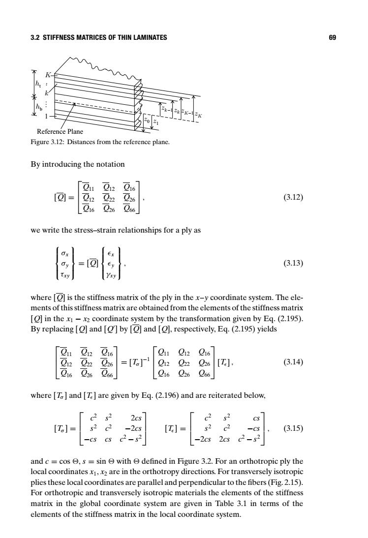
3.2 STIFFNESS MATRICES OF THIN LAMINATES 69 Reference Plane Figure 3.12:Distances from the reference plane. By introducing the notation Cu 012 216 [Q]= Q12 022 026 (3.12) ②16 026 266 we write the stress-strain relationships for a ply as (3.13) where [O is the stiffness matrix of the ply in the x-y coordinate system.The ele- ments of this stiffness matrix are obtained from the elements of the stiffness matrix [O]in the xi-x2 coordinate system by the transformation given by Eq.(2.195) By replacing [O]and [O]by [O]and [O],respectively,Eq.(2.195)yields 11 On O Q11 Q12 Q16 12 6 =[T] Q12 Q22 Q26 (3.14) 亘26 O66 Q16 Q26 Q66 where [T and [T]are given by Eq.(2.196)and are reiterated below, c2 2es c2 s2 cs [T]= -2cs [T]= s2 c2 -CS (3.15) 一CS cs c2-s2 -2cs 2cs c2-s2 and c cos s sin with defined in Figure 3.2.For an orthotropic ply the local coordinates x1,x2 are in the orthotropy directions.For transversely isotropic plies these local coordinates are parallel and perpendicular to the fibers(Fig.2.15) For orthotropic and transversely isotropic materials the elements of the stiffness matrix in the global coordinate system are given in Table 3.1 in terms of the elements of the stiffness matrix in the local coordinate system.3.2 STIFFNESS MATRICES OF THIN LAMINATES 69 Reference Plane ht hb K … 1.. zk –1 zk zK–1 z1 zK z0 k Figure 3.12: Distances from the reference plane. By introducing the notation [Q] =    Q11 Q12 Q16 Q12 Q22 Q26 Q16 Q26 Q66    , (3.12) we write the stress–strain relationships for a ply as    σx σy τxy    = [Q]    x y γxy    , (3.13) where [Q] is the stiffness matrix of the ply in the x–y coordinate system. The ele￾ments of this stiffness matrix are obtained from the elements of the stiffness matrix [Q] in the x1 − x2 coordinate system by the transformation given by Eq. (2.195). By replacing [Q] and [Q ] by [Q] and [Q], respectively, Eq. (2.195) yields    Q11 Q12 Q16 Q12 Q22 Q26 Q16 Q26 Q66    = [Tσ ] −1    Q11 Q12 Q16 Q12 Q22 Q26 Q16 Q26 Q66    [T ] , (3.14) where [Tσ ] and [T ] are given by Eq. (2.196) and are reiterated below, [Tσ ] =    c2 s2 2cs s2 c2 −2cs −cs cs c2 − s2    [T ] =    c2 s2 cs s2 c2 −cs −2cs 2cs c2 − s2    , (3.15) and c = cos , s = sin  with  defined in Figure 3.2. For an orthotropic ply the local coordinates x1, x2 are in the orthotropy directions. For transversely isotropic plies these local coordinates are parallel and perpendicular to the fibers (Fig. 2.15). For orthotropic and transversely isotropic materials the elements of the stiffness matrix in the global coordinate system are given in Table 3.1 in terms of the elements of the stiffness matrix in the local coordinate system.