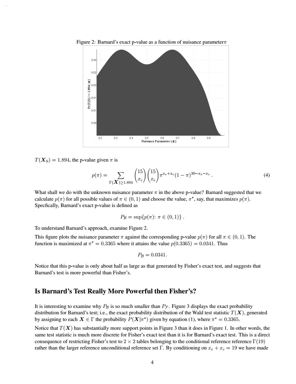
Figure 2:Barnard's exact p-value as a function of nuisance parameterm 002 002 001 000 02 04 05 0.6 07 0.8 0.9 Nuisance Parameter (x) T(Xo)=1.894,the p-value given m is p()=∑ 15 /15 2ete(1-)30-e-e. (4) T(X)≥1.894 What shall we do with the unknown nuisance parameter m in the above p-value?Barnard suggested that we calculate p(π)for all possible values of∈(0，l)and choose the value,.π*，say,that maximizes p(π). Specfically,Barnard's exact p-value is defined as Ps=supp(π：T∈(0,1)}. To understand Barnard's approach,examine Figure 2. This figure plots the nuisance parameter m against the corresponding p-value p()for all E(0,1).The function is maximized at *=0.3365 where it attains the value p(0.3365)=0.0341.Thus P6=0.0341. Notice that this p-value is only about half as large as that generated by Fisher's exact test,and suggests that Barnard's test is more powerful than Fisher's. Is Barnard's Test Really More Powerful then Fisher's? It is interesting to examine why PB is so much smaller than PF.Figure 3 displays the exact probability distribution for Barnard's test;i.e.,the exact probability distribution of the Wald test statistic T(X),generated by assigning to each X EI the probability P(X*)given by equation (1),where n*=0.3365. Notice that T(X)has substantially more support points in Figure 3 than it does in Figure 1.In other words,the same test statistic is much more discrete for Fisher's exact test than it is for Barnard's exact test.This is a direct consequence of restricting Fisher's test to 2 x 2 tables belonging to the conditional reference reference I(19) rather than the larger reference unconditional reference set I.By conditioning on ze+e=19 we have made 4Figure 2: Barnard’s exact p-value as a function of nuisance parameterπ T(X0)=1.894, the p-value given π is p(π) = T(X)≥1.894
15 xc
15 xe πxe+xc (1 − π) 30−xe−xc . (4) What shall we do with the unknown nuisance parameter π in the above p-value? Barnard suggested that we calculate p(π) for all possible values of π ∈ (0, 1) and choose the value, π∗, say, that maximizes p(π). Specfically, Barnard’s exact p-value is defined as PB = sup{p(π): π ∈ (0, 1)} . To understand Barnard’s approach, examine Figure 2. This figure plots the nuisance parameter π against the corresponding p-value p(π) for all π ∈ (0, 1). The function is maximized at π∗ = 0.3365 where it attains the value p(0.3365) = 0.0341. Thus PB = 0.0341. Notice that this p-value is only about half as large as that generated by Fisher’s exact test, and suggests that Barnard’s test is more powerful than Fisher’s. Is Barnard’s Test Really More Powerful then Fisher’s? It is interesting to examine why PB is so much smaller than PF . Figure 3 displays the exact probability distribution for Barnard’s test; i.e., the exact probability distribution of the Wald test statistic T(X), generated by assigning to each X ∈ Γ the probability P(X|π∗) given by equation (1), where π∗ = 0.3365. Notice that T(X) has substantially more support points in Figure 3 than it does in Figure 1. In other words, the same test statistic is much more discrete for Fisher’s exact test than it is for Barnard’s exact test. This is a direct consequence of restricting Fisher’s test to 2 × 2 tables belonging to the conditional reference reference Γ(19) rather than the larger reference unconditional reference set Γ. By conditioning on xe + xc = 19 we have made 4