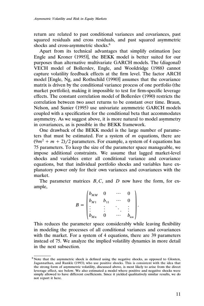
Asymmetric Volatility and Risk in Equity Markets return are related to past conditional variances and covariances,past squared residuals and cross residuals,and past squared asymmetric shocks and cross-asymmetric shocks. Apart from its technical advantages that simplify estimation [see Engle and Kroner (1995)],the BEKK model is better suited for our purposes than alternative multivariate GARCH models.The (diagonal) VECH model of Bollerslev,Engle,and Wooldridge (1988)cannot capture volatility feedback effects at the firm level.The factor ARCH model [Engle,Ng,and Rothschild (1990)]assumes that the covariance matrix is driven by the conditional variance process of one portfolio (the market portfolio),making it impossible to test for firm-specific leverage effects.The constant correlation model of Bollerslev (1990)restricts the correlation between two asset returns to be constant over time.Braun, Nelson,and Sunier (1995)use univariate asymmetric GARCH models coupled with a specification for the conditional beta that accommodates asymmetry.As we suggest above,it is more natural to model asymmetry in covariances,as is possible in the BEKK framework. One drawback of the BEKK model is the large number of parame- ters that must be estimated.For a system of m equations,there are (9m2+m 2)/2 parameters.For example,a system of 4 equations has 75 parameters.To keep the size of the parameter space manageable,we impose additional constraints.We assume that lagged market-level shocks and variables enter all conditional variance and covariance equations,but that individual portfolio shocks and variables have ex- planatory power only for their own variances and covariances with the market. The parameter matrices B,C,and D now have the form,for ex- ample, DMM 0 0 B= bMn 0 This reduces the parameter space considerably while leaving flexibility in modeling the processes of all conditional variances and covariances with the market.For a system of 4 equations,there are 39 parameters instead of 75.We analyze the implied volatility dynamics in more detail in the next subsection. 6 Note that the asymmetric shock is defined using the negative shocks,as opposed to Glosten. Jagannathan,and Runkle (1993),who use positive shocks.This is consistent with the idea that the strong form of asymmetric volatility,discussed above,is most likely to arise from the direct leverage effect,see below.We also estimated a model where positive and negative shocks were simply allowed to have different coefficients.Since it yielded qualitatively similar results,we do not report it here. 11Asymmetric Volatility and Risk in Equity Markets return are related to past conditional variances and covariances, past squared residuals and cross residuals, and past squared asymmetric shocks and cross-asymmetric shocks.6 Apart from its technical advantages that simplify estimation see
Engle and Kroner 1995 , the BEKK model is better suited for our Ž . purposes than alternative multivariate GARCH models. The diagonal Ž . VECH model of Bollerslev, Engle, and Wooldridge 1988 cannot Ž . capture volatility feedback effects at the firm level. The factor ARCH model Engle, Ng, and Rothschild 1990 assumes that the covariance
Ž . matrix is driven by the conditional variance process of one portfolio the Ž market portfolio , making it impossible to test for firm-specific leverage . effects. The constant correlation model of Bollerslev 1990 restricts the Ž . correlation between two asset returns to be constant over time. Braun, Nelson, and Sunier 1995 use univariate asymmetric GARCH models Ž . coupled with a specification for the conditional beta that accommodates asymmetry. As we suggest above, it is more natural to model asymmetry in covariances, as is possible in the BEKK framework. One drawback of the BEKK model is the large number of parame￾ters that must be estimated. For a system of m equations, there are Ž 2 9m  m  2.2 parameters. For example, a system of 4 equations has 75 parameters. To keep the size of the parameter space manageable, we impose additional constraints. We assume that lagged market-level shocks and variables enter all conditional variance and covariance equations, but that individual portfolio shocks and variables have ex￾planatory power only for their own variances and covariances with the market. The parameter matrices B, C, and D now have the form, for ex￾ample, bM M 0  0 b b M 1 11  0 B  . .. . . . . .. . . ..  0 bMn nn 0  b This reduces the parameter space considerably while leaving flexibility in modeling the processes of all conditional variances and covariances with the market. For a system of 4 equations, there are 39 parameters instead of 75. We analyze the implied volatility dynamics in more detail in the next subsection. 6 Note that the asymmetric shock is defined using the negative shocks, as opposed to Glosten, Jagannathan, and Runkle 1993 , who use positive shocks. This is consistent with the idea that Ž . the strong form of asymmetric volatility, discussed above, is most likely to arise from the direct leverage effect, see below. We also estimated a model where positive and negative shocks were simply allowed to have different coefficients. Since it yielded qualitatively similar results, we do not report it here. 11