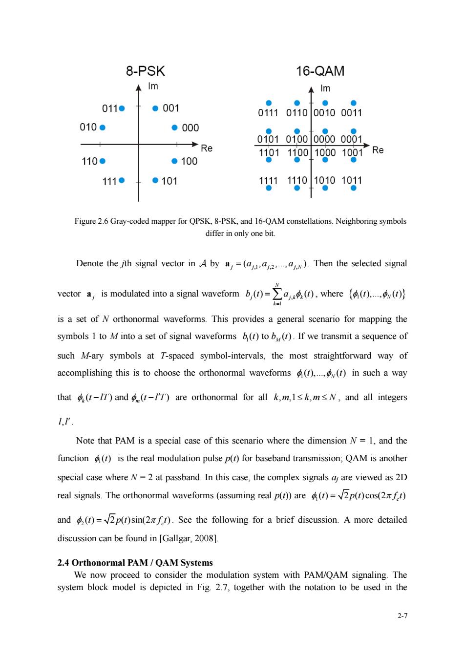
8-PSK 16-QAM ↑m ←lm 011● ●001 01i101i00010o0i1 010● ●000 Re 0101010000000001. 110● ●100 1101110010o01o07Re 111● ●101 111110101010g1 Figure 26 Gray-coded mapper for QPSK.8-PSK.and 16-QAM constellations.Neighboring symbols differ in only one bit. Denote the jth signal vector in A by a,=(a).Then the selected signal is a set of N orthonormal waveforms.This provides a general scenario for mapping the symbols I to M into a set of signal waveforms b(r)to b().If we transmit a sequence of such M-ary symbols at T-spaced symbol-intervals,the most straightforward way of accomplishing this is to choose the orthonormal waveforms).(t)in such a way that-T)and (-/'T)are orthonormal for all k,m,Isk,m<N,and all integers Note that PAM is a special case of this scenario where the dimension N=1,and the function)is the real modulation pulse p(r)for baseband transmission:QAM is another special case where N=2 at passband.In this case,the complex signals a are viewed as 2D real signals.The orthonormal waveforms (assuming real p())are)=2p()cos(2) and()=2p(r)sin(f).See the following for a brief discussion.A more detailed discussion can be found in [Gallgar,200] 2.4 Orthonormal PAM/QAM Systems We now proceed to consider the modulation system with PAM/QAM signaling.The system block model is depicted in Fig.2.7.together with the notation to be used in the 22-7 Figure 2.6 Gray-coded mapper for QPSK, 8-PSK, and 16-QAM constellations. Neighboring symbols differ in only one bit. Denote the jth signal vector in  by ,1 ,2 , ( , ,., ) j j j j N a = a a a . Then the selected signal vector j a is modulated into a signal waveform , 1 ( ) ( ) N j j k k k b t a t  = =  , where   1 ( ),., ( ) t t N  is a set of N orthonormal waveforms. This provides a general scenario for mapping the symbols 1 to M into a set of signal waveforms 1 ( ) to ( ) M b t b t . If we transmit a sequence of such M-ary symbols at T-spaced symbol-intervals, the most straightforward way of accomplishing this is to choose the orthonormal waveforms 1 ( ),., ( ) N   t t in such a way that ( ) and ( ) k m   t lT t l T − −  are orthonormal for all k m k m N , ,1 ,   , and all integers ll, . Note that PAM is a special case of this scenario where the dimension N = 1, and the function 1  ()t is the real modulation pulse p(t) for baseband transmission; QAM is another special case where N = 2 at passband. In this case, the complex signals aj are viewed as 2D real signals. The orthonormal waveforms (assuming real p(t)) are 1 ( ) 2 ( )cos(2 ) c   t p t f t = and 2 ( ) 2 ( )sin(2 ) c   t p t f t = . See the following for a brief discussion. A more detailed discussion can be found in [Gallgar, 2008]. 2.4 Orthonormal PAM / QAM Systems We now proceed to consider the modulation system with PAM/QAM signaling. The system block model is depicted in Fig. 2.7, together with the notation to be used in the