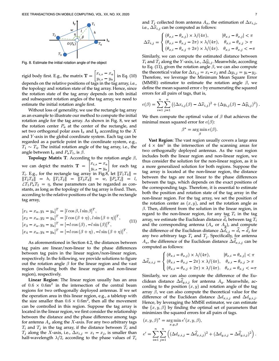
IEEE TRANSACTIONS ON MOBILE COMPUTING,VOL.XX,NO.XX,2020 and T;collected from antenna Ar,the estimation of Ari.j, i.e.,Aij can be computed as follows: (0z,i-0z,)×/(4r), l9z,i-6x<元 △i,= (0x,i-8x-2r)×/(4π)，8z,i-0z.>π (0x,i-9x,+2r)×/(4π).8x,i-0z,j<-π Similarly,we can compute the estimated distance between Fig.8.Estimate the initial rotation angle of the object Ti and Ti along the Y-axis,i.e.,Ati.j.Meanwhile,according to Eq.(11),given the rotation angle B,we can also compute rigid body first.E.g.,the matrix T= Ti,s-Ta the theoretical value for Ari.j =i-xj and Ayi.j=yi-yj. yi,s-Ya in Eg.(10) Therefore,we leverage the Minimum Mean Square Error depends on the relative positions of tags in the tag array,i.e., (MMSE)estimator to estimate the rotation angle B,we the topology and rotation state of the tag array.Hence,since define the mean squared error e by enumerating the squared the rotation state of the tag array depends on both initial errors for all pairs of tags,that is, and subsequent rotation angles of the tag array,we need to estimate the initial rotation angle first. e(B)= ∑∑（△r()-△立）2+（△(）-△P) Without loss of generality,we use the rectangle tag array i=1j=1 as an example to illustrate our method to compute the initial We then compute the optimal value of B that achieves the rotation angle for the tag array.As shown in Fig.8,we set minimal mean squared error for e(B): the rotation center Pa at the center of the rectangle,and set two orthogonal polar axes l and ly according to the X B*=arg min e(B). and Y-axis in the global coordinate system.Each tag can be regarded as a particle point in the coordinate system,e.g., Vast Region:The vast region usually covers a large area T~T4.The initial rotation angle of the tag array,i.e.,the of 4 x 4m2 in the intersection of the scanning areas for angle between Ir and PaT1,is B. two orthogonally deployed antennas.As the vast region Topology Matrix T.According to the rotation angle B, includes both the linear region and non-linear region,we Ti,s-Ta thus consider the solution for the non-linear region,as it is we can depict the matrix T for each tag Yi.8-Ya a more generalized solution for both regions.Suppose the Ti.E.g.,for the rectangle tag array in Fig.8,let TiTall tag array is located at the non-linear region,the distance T2T3ll h,ITT2ll IT3Tll w,PaTill L, between the tags are not linear to the phase differences LT1PaT2 =n,these parameters can be regarded as con- between the tags,which depends on the exact positions of stants,as long as the topology of the tag array is fixed.Then, the corresponding tags.Therefore,it is essential to estimate according to the relative positions of the tags in the rectangle both the position and rotation state of the tag array in the tag array, non-linear region.For the tag array,we set the position of the rotation center as (x,y),and set the rotation angle as [1-za:y-ya]T=[l cos B,Isin B]T, B.Then,different from the solution in the linear region,in [2-a:y2-ya]T=[l cos(8+n),Isin (8+n)], regard to the non-linear region,for any tag Ti in the tag array,we estimate the Euclidean distance di between tag Ti [s-za:U3-ya]T=[-lcos(B),-Isin (B)]T, (11) and the corresponding antenna(A-or Ay),and compute [z4-xa,4-aT=【-lcos(B+n),-lsin(B+nj】T the difference of the Euclidean distance Adi.j=di-dj for any two arbitrary tags Ti and Ti.Specifically,for antenna As aforementioned in Section 4.2,the distances between Ar,the difference of the Euclidean distance Adr.i.j can be tag pairs are linear/non-linear to the phase differences computed as follows: between tag pairs in the linear region/non-linear region, (0z,i-0z,）×入/(4π)： 10zi-0z.jl<T respectively.In the following,we provide solutions to figure out the rotation angle B for the linear region and the vast △dzij (0x,i-0z.-2r）×λ/（4r),0x.i-0z,j>T region (including both the linear region and non-linear (0z,i-0x,1+2x）×λ/(4r).0z,i-8x,<-元 region),respectively. Similarly,we can also compute the difference of the Eu- Linear Region:The linear region usually has an area clidean distance Ady.i.j for antenna Ay.Meanwhile,ac- of 0.6 x 0.6m2 in the intersection of the central beam cording to the position (x,y)and rotation angle of the tag regions for two orthogonally deployed antennas.If we set array B,we can also compute the theoretical value for the the operation area in this linear region,e.g.,a tabletop with difference of the Euclidean distance Adz.i.j and Ady.i.j. the size smaller than 0.6 x 0.6m2,then all the movement Hence,by leveraging the MMSE estimator,we can estimate can be controlled in this region.Suppose the tag array is the,,B}by finding the optimal set of parameters that located in the linear region,we first consider the relationship minimizes the squared errors for all pairs of tags. between the distance and the phase difference among tags for antenna Ar along the X-axis.For any two arbitrary tags (,y,B)"=arg min e'(,y,B), Ti and Tj in the tag array,if the distance between Ti and x,y,8 Tj along the X-axis,i.e.,Axi.j ri-xj,is smaller than half-wavelength A/2,according to the phase values of Ti e=∑∑（ad-△dP+(ad,-△d,P) 11IEEE TRANSACTIONS ON MOBILE COMPUTING, VOL. XX, NO. XX, 2020 7 ܶଵ ȟݔଵଶ ܶଶ ܶଷ ܶସ ȟݕଵଶ ߚ ଷସݔȟ ߚ ȟݕଷସ ܶଵ ܶଶ ܶଷ ܶସ ߚ ݈ ݓ ݄ ߟ ܱ(ܲ௔) ܠܔ ܡܔ Fig. 8. Estimate the initial rotation angle of the object rigid body first. E.g., the matrix T =  xi,s − xa yi,s − ya  in Eq. (10) depends on the relative positions of tags in the tag array, i.e., the topology and rotation state of the tag array. Hence, since the rotation state of the tag array depends on both initial and subsequent rotation angles of the tag array, we need to estimate the initial rotation angle first. Without loss of generality, we use the rectangle tag array as an example to illustrate our method to compute the initial rotation angle for the tag array. As shown in Fig. 8, we set the rotation center Pa at the center of the rectangle, and set two orthogonal polar axes lx and ly according to the X and Y -axis in the global coordinate system. Each tag can be regarded as a particle point in the coordinate system, e.g., T1 ∼ T4. The initial rotation angle of the tag array, i.e., the angle between lx and PaT1, is β. Topology Matrix T. According to the rotation angle β, we can depict the matrix T =  xi,s − xa yi,s − ya  for each tag Ti . E.g., for the rectangle tag array in Fig.8, let kT1T4k = kT2T3k = h, kT1T2k = kT3T4k = w, kPaTik = l, 6 T1PaT2 = η, these parameters can be regarded as con￾stants, as long as the topology of the tag array is fixed. Then, according to the relative positions of the tags in the rectangle tag array, [x1 − xa, y1 − ya] T = [l cos β, lsin β] T , [x2 − xa, y2 − ya] T = [l cos (β + η), lsin (β + η)]T , [x3 − xa, y3 − ya] T = [−l cos (β), −lsin (β)]T , [x4 − xa, y4 − ya] T = [−l cos (β + η), −lsin (β + η)]T . (11) As aforementioned in Section 4.2, the distances between tag pairs are linear/non-linear to the phase differences between tag pairs in the linear region/non-linear region, respectively. In the following, we provide solutions to figure out the rotation angle β for the linear region and the vast region (including both the linear region and non-linear region), respectively. Linear Region: The linear region usually has an area of 0.6 × 0.6m2 in the intersection of the central beam regions for two orthogonally deployed antennas. If we set the operation area in this linear region, e.g., a tabletop with the size smaller than 0.6 × 0.6m2 , then all the movement can be controlled in this region. Suppose the tag array is located in the linear region, we first consider the relationship between the distance and the phase difference among tags for antenna Ax along the X-axis. For any two arbitrary tags Ti and Tj in the tag array, if the distance between Ti and Tj along the X-axis, i.e., ∆xi,j = xi − xj , is smaller than half-wavelength λ/2, according to the phase values of Ti and Tj collected from antenna Ax, the estimation of ∆xi,j , i.e., ∆xbi,j can be computed as follows: ∆xbi,j =    (θx,i − θx,j ) × λ/(4π), |θx,i − θx,j | < π (θx,i − θx,j − 2π) × λ/(4π), θx,i − θx,j > π (θx,i − θx,j + 2π) × λ/(4π). θx,i − θx,j < −π Similarly, we can compute the estimated distance between Ti and Tj along the Y -axis, i.e., ∆ybi,j . Meanwhile, according to Eq. (11), given the rotation angle β, we can also compute the theoretical value for ∆xi,j = xi−xj and ∆yi,j = yi−yj . Therefore, we leverage the Minimum Mean Square Error (MMSE) estimator to estimate the rotation angle β, we define the mean squared error e by enumerating the squared errors for all pairs of tags, that is, e(β) = Xn i=1 Xn j=1 ￾ (∆xi,j (β) − ∆xbi,j ) 2 + (∆yi,j (β) − ∆ybi,j ) 2
. We then compute the optimal value of β that achieves the minimal mean squared error for e(β): β ∗ = arg min β e(β). Vast Region: The vast region usually covers a large area of 4 × 4m2 in the intersection of the scanning areas for two orthogonally deployed antennas. As the vast region includes both the linear region and non-linear region, we thus consider the solution for the non-linear region, as it is a more generalized solution for both regions. Suppose the tag array is located at the non-linear region, the distance between the tags are not linear to the phase differences between the tags, which depends on the exact positions of the corresponding tags. Therefore, it is essential to estimate both the position and rotation state of the tag array in the non-linear region. For the tag array, we set the position of the rotation center as (x, y), and set the rotation angle as β. Then, different from the solution in the linear region, in regard to the non-linear region, for any tag Ti in the tag array, we estimate the Euclidean distance dbi between tag Ti and the corresponding antenna (Ax or Ay), and compute the difference of the Euclidean distance ∆dbi,j = dbi − dbj for any two arbitrary tags Ti and Tj . Specifically, for antenna Ax, the difference of the Euclidean distance ∆dbx,i,j can be computed as follows: ∆dbx,i,j =    (θx,i − θx,j ) × λ/(4π), |θx,i − θx,j | < π (θx,i − θx,j − 2π) × λ/(4π), θx,i − θx,j > π (θx,i − θx,j + 2π) × λ/(4π). θx,i − θx,j < −π Similarly, we can also compute the difference of the Eu￾clidean distance ∆dby,i,j for antenna Ay. Meanwhile, ac￾cording to the position (x, y) and rotation angle of the tag array β, we can also compute the theoretical value for the difference of the Euclidean distance ∆dx,i,j and ∆dy,i,j . Hence, by leveraging the MMSE estimator, we can estimate the {x, y, β} by finding the optimal set of parameters that minimizes the squared errors for all pairs of tags. (x, y, β) ∗ = arg min x,y,β e 0 (x, y, β), e 0 = Xn i=1 Xn j=1  (∆dx,i,j − ∆dbx,i,j ) 2 + (∆dy,i,j − ∆dby,i,j ) 2