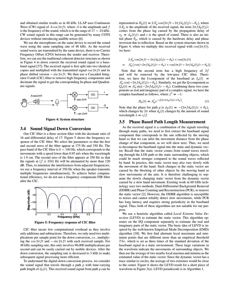
and obtained similar results as in 48 kHz.LLAP uses Continuous represented as Rp(t)=2A cos(2rft-2nfdp(t)/c-0p).where Wave(CW)signal of Acos 2ft,where A is the amplitude and f 2Ap is the amplitude of the received signal,the term 2fdp(t)/c is the frequency of the sound,which is in the range of 1723 kHz. comes from the phase lag caused by the propagation delay of CW sound signals in this range can be generated by many COTS Tp =dp(t)/c and c is the speed of sound.There is also an ini- devices without introducing audible noises [6]. tial phase p.which is caused by the hardware delay and phase We use the microphones on the same device to record the sound inversion due to reflection.Based on the system structure shown in wave using the same sampling rate of 48 kHz.As the received Figure 4,when we multiply this received signal with cos(2ft) sound waves are transmitted by the same device,there is no Carrier we have: Frequency Offset(CFO)between the sender and receiver.There- fore.we can use the traditional coherent detector structure as shown 2 A cos(2rft-2πfdp(t)/c-0p)×cos(2πft) in Figure 4 to down convert the received sound signal to a base- band signal [37].The received signal is first split into two identical Ap(cos(-2xfdp(t)/c-0p)+cos(4nft-2mfdp(t)/c-0p)). copies and multiplied with the transmitted signal cos 2ft and its Note that the second term has a high frequency of 2f phase shifted version-sin 2mft.We then use a Cascaded Integ- and will be removed by the low-pass CIC filter.There- rator Comb(CIC)filter to remove high frequency components and fore,we have the I-component of the baseband as Ip(t)= decimate the signal to get the corresponding In-phase and Quadrat- Ap cos(-2rfdp(t)/c-0p).Similarly,we get the Q-component as ure signals. Qp(t)=Ap sin(-2fdp(t)/c-0p).Combining these two com- ponents as real and imaginary part of a complex signal,we have the Acos2nft CIC complex baseband as follows,wherej=-1: ↑cos2mft Bp(t)=Ate-i(2x/dp(t)/c+0p) (1) Q CIC Note that the phase for path p is p(t)=-(2xfdp(t)/c+p). ↑-sin2mft which changes by 2 when dp(t)changes by the amount of sound wavelength入=c/f Figure 4:System structure 3.5 Phase Based Path Length Measurement 3.4 Sound Signal Down Conversion As the received signal is a combination of the signals traveling through many paths,we need to first extract the baseband signal Our CIC filter is a three section filter with the decimate ratio of component that corresponds to the one reflected by the moving 16 and differential delay of 17.Figure 5 shows the frequency re- hand so that we can infer the movement distance from the phase sponse of the CIC filter.We select the parameters so that the first change of that component,as we will show next.Thus.we need and second zeros of the filter appear at 175 Hz and 350 Hz.The to decompose the baseband signal into the static and dynamic vec- pass-band of the CIC filter is0100 Hz,which corresponds to the tor.Recall that the static vector comes from sound waves travel- movements with a speed lower than 0.95 m/s when the wavelength ing through the LOS path or the static surrounding objects,which is 1.9 cm.The second zero of the filter appears at 350 Hz so that could be much stronger compared to the sound waves reflected the signals at (f+350)Hz will be attenuated by more than 120 by hand.In practice,this static vector may also vary slowly with dB.Thus,to minimize the interferences from adjacent frequencies. the movement of the hand.Such changes in the static vector are we use a frequency interval of 350 Hz when the speaker transmits caused by the blocking of other objects by the moving hand or multiple frequencies simultaneously.To achieve better computa- slow movements of the arm.It is therefore challenging to sep- tional efficiency,we do not use a frequency compensate FIR filter arate the slowly changing static vector from the dynamic vector after the CIC. caused by a slow hand movement.Existing work in 60 GHz tech- nology uses two methods.Dual-Differential Background Removal (DDBR)and Phase Counting and Reconstruction(PCR).to remove -与0 the static vector [2].However,the DDBR algorithm is susceptible to noises and cannot reliably detect slow movements,while PCR 100 has long latency and requires strong periodicity in the baseband signal.Thus,both of these algorithms are not suitable for our pur- .150 pose. 0正 0 0.8 We use a heuristic algorithm called Local Extreme Value De- Frequency(kHz) tection (LEVD)to estimate the static vector.This algorithm op Figure 5:Frequency response of CIC filter erates on the I/Q component separately to estimate the real and imaginary parts of the static vector.The basic idea of LEVD is in- CIC filter incurs low computational overhead as they involve spired by the well-known Empirical Mode Decomposition (EMD) only additions and subtractions.Therefore,we only need two multi- algorithm [38].We first find alternate local maximum and min- plications per sample point for the down conversion,i.e..multiply- imum points that are different more than an empirical threshold ing the cos 2mft and -sin 2ft with each received sample.For Thr,which is set as three times of the standard deviation of the 48 kHz sampling rate,this only involves 96,000 multiplications per baseband signal in a static environment.These large variations in second and can be easily carried out by mobile devices.After the the waveform indicate the movements of surrounding objects.We down conversion,the sampling rate is decreased to 3 kHz to make then use the average of two nearby local maxima and minima as the subsequent signal processing more efficient. estimated value of the static vector.Since the dynamic vector has a To understand the digital down conversion process,we consider trace similar to circles,the average of two extremes would be close the sound signal that travels through a path p with time-varying to the center.Figure 6 shows the LEVD result for a short piece of path length of dp(t).This received sound signal from path p can be waveform in Figure 3(a).LEVD pseudocode is in Algorithm 1.and obtained similar results as in 48 kHz. LLAP uses Continuous Wave (CW) signal of A cos 2πf t, where A is the amplitude and f is the frequency of the sound, which is in the range of 17 ∼ 23 kHz. CW sound signals in this range can be generated by many COTS devices without introducing audible noises [6]. We use the microphones on the same device to record the sound wave using the same sampling rate of 48 kHz. As the received sound waves are transmitted by the same device, there is no Carrier Frequency Offset (CFO) between the sender and receiver. There￾fore, we can use the traditional coherent detector structure as shown in Figure 4 to down convert the received sound signal to a base￾band signal [37]. The received signal is first split into two identical copies and multiplied with the transmitted signal cos 2πf t and its phase shifted version − sin 2πf t. We then use a Cascaded Integ￾rator Comb (CIC) filter to remove high frequency components and decimate the signal to get the corresponding In-phase and Quadrat￾ure signals. cos 2πft —sin 2πft CIC CIC I Q Acos2πft Figure 4: System structure 3.4 Sound Signal Down Conversion Our CIC filter is a three section filter with the decimate ratio of 16 and differential delay of 17. Figure 5 shows the frequency re￾sponse of the CIC filter. We select the parameters so that the first and second zeros of the filter appear at 175 Hz and 350 Hz. The pass-band of the CIC filter is 0 ∼ 100 Hz, which corresponds to the movements with a speed lower than 0.95 m/s when the wavelength is 1.9 cm. The second zero of the filter appears at 350 Hz so that the signals at (f ± 350) Hz will be attenuated by more than 120 dB. Thus, to minimize the interferences from adjacent frequencies, we use a frequency interval of 350 Hz when the speaker transmits multiple frequencies simultaneously. To achieve better computa￾tional efficiency, we do not use a frequency compensate FIR filter after the CIC. 0 0.2 0.4 0.6 0.8 1 −150 −100 −50 0 Frequency (kHz) Magnitude (dB) Figure 5: Frequency response of CIC filter CIC filter incurs low computational overhead as they involve only additions and subtractions. Therefore, we only need two multi￾plications per sample point for the down conversion, i.e., multiply￾ing the cos 2πf t and − sin 2πf t with each received sample. For 48 kHz sampling rate, this only involves 96,000 multiplications per second and can be easily carried out by mobile devices. After the down conversion, the sampling rate is decreased to 3 kHz to make subsequent signal processing more efficient. To understand the digital down conversion process, we consider the sound signal that travels through a path p with time-varying path length of dp(t). This received sound signal from path p can be represented as Rp(t) = 2A 0 p cos(2πf t−2πf dp(t)/c−θp), where 2A 0 p is the amplitude of the received signal, the term 2πf dp(t)/c comes from the phase lag caused by the propagation delay of τp = dp(t)/c and c is the speed of sound. There is also an ini￾tial phase θp, which is caused by the hardware delay and phase inversion due to reflection. Based on the system structure shown in Figure 4, when we multiply this received signal with cos(2πf t), we have: 2A 0 p cos(2πf t − 2πf dp(t)/c − θp) × cos(2πf t) = A 0 p ￾ cos(−2πf dp(t)/c − θp) + cos(4πf t − 2πf dp(t)/c − θp)
. Note that the second term has a high frequency of 2f and will be removed by the low-pass CIC filter. There￾fore, we have the I-component of the baseband as Ip(t) = A 0 p cos(−2πf dp(t)/c−θp). Similarly, we get the Q-component as Qp(t) = A 0 p sin(−2πf dp(t)/c − θp). Combining these two com￾ponents as real and imaginary part of a complex signal, we have the complex baseband as follows, where j 2 = −1: Bp(t) = A 0 pe −j(2πfdp(t)/c+θp) . (1) Note that the phase for path p is φp(t) = −(2πf dp(t)/c + θp), which changes by 2π when dp(t) changes by the amount of sound wavelength λ = c/f. 3.5 Phase Based Path Length Measurement As the received signal is a combination of the signals traveling through many paths, we need to first extract the baseband signal component that corresponds to the one reflected by the moving hand so that we can infer the movement distance from the phase change of that component, as we will show next. Thus, we need to decompose the baseband signal into the static and dynamic vec￾tor. Recall that the static vector comes from sound waves travel￾ing through the LOS path or the static surrounding objects, which could be much stronger compared to the sound waves reflected by hand. In practice, this static vector may also vary slowly with the movement of the hand. Such changes in the static vector are caused by the blocking of other objects by the moving hand or slow movements of the arm. It is therefore challenging to sep￾arate the slowly changing static vector from the dynamic vector caused by a slow hand movement. Existing work in 60 GHz tech￾nology uses two methods, Dual-Differential Background Removal (DDBR) and Phase Counting and Reconstruction (PCR), to remove the static vector [2]. However, the DDBR algorithm is susceptible to noises and cannot reliably detect slow movements, while PCR has long latency and requires strong periodicity in the baseband signal. Thus, both of these algorithms are not suitable for our pur￾pose. We use a heuristic algorithm called Local Extreme Value De￾tection (LEVD) to estimate the static vector. This algorithm op￾erates on the I/Q component separately to estimate the real and imaginary parts of the static vector. The basic idea of LEVD is in￾spired by the well-known Empirical Mode Decomposition (EMD) algorithm [38]. We first find alternate local maximum and min￾imum points that are different more than an empirical threshold T hr, which is set as three times of the standard deviation of the baseband signal in a static environment. These large variations in the waveform indicate the movements of surrounding objects. We then use the average of two nearby local maxima and minima as the estimated value of the static vector. Since the dynamic vector has a trace similar to circles, the average of two extremes would be close to the center. Figure 6 shows the LEVD result for a short piece of waveform in Figure 3(a). LEVD pseudocode is in Algorithm 1