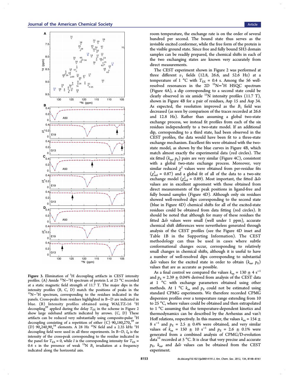
Joural of the American Chemical Society Article A 75 be ready known very accurately from eo1cD g the 56 well. ces in the )a dip 130 125 118110 in Fig the profiles (11.7 T) d as the B the tra 1at26 ad fit p es ach of the an a d in the E19 ave bee fit to odel,as sho in ta a Pro ess Mo bal fit of all of the ange mod 0.89).Most 4D)ch of well u the Figu E19 ed in case nge ,G13 ll-resolved ding to su 10 125 d the valu 1304 obtained usins other that the by th (D)of a and 2.5±0.4% tained. nd y simila ty ing to th It is de tha very pre e ar 815 delere/10 1021/30014191 Am.Chem.Sec.2012.134.8168-816room temperature, the exchange rate is on the order of several hundred per second. The bound state thus serves as the invisible excited conformer, while the free form of the protein is the visible ground state. Since free and fully bound SH3 domain samples can be readily prepared, the chemical shifts in each of the two exchanging states are known very accurately from direct measurements. The CEST experiment shown in Figure 2 was performed at three different ν1 fields (12.8, 26.6, and 52.6 Hz) at a temperature of 1 °C with TEX = 0.4 s. Among the 56 well￾resolved resonances in the 2D 15N−1 H HSQC spectrum (Figure 4A), a dip corresponding to a second state could be clearly observed in six amide 15N intensity profiles (11.7 T), shown in Figure 4B for a pair of residues, Asp 15 and Asp 34. As expected, the resolution improved as the B1 field was decreased (as seen by comparison of the traces recorded at 26.6 and 12.8 Hz). Rather than assuming a global two-state exchange process, we instead fit profiles from each of the six residues independently to a two-state model. If an additional dip, corresponding to a third state, had been observed in the CEST profiles, the data would have been fit to a three-state exchange mechanism. Excellent fits were obtained with the two￾state model, as shown by the blue curves in Figure 4B, which match almost exactly the experimental data (red circles). The six fitted (kex, pE) pairs are very similar (Figure 4C), consistent with a global two-state exchange process. Moreover, very similar reduced χ2 values were obtained from per-residue fits (χred 2 = 0.87) and a global fit of all of the data to a two-site exchange model (χred 2 = 0.89). Most important, the fitted Δω̃ values are in excellent agreement with those obtained from direct measurements of the peak positions in ligand-free and fully bound samples (Figure 4D). Although only six residues showed well-resolved dips corresponding to the second state (blue in Figure 4D) chemical shifts for all of the excited-state residues could be obtained from data fitting (red circles). It should be noted that although for many of these residues the fitted Δω̃ values were small (well under 1 ppm), accurate chemical shift differences were nevertheless generated through analysis of the CEST profiles (see the Figure 4D inset and Table 1B in the Supporting Information). The CEST methodology can thus be used in cases where subtle conformational changes occur, corresponding to relatively small changes in chemical shifts, although it is useful to have a number of well-resolved dips corresponding to substantial Δω̃ values for the excited state in order to obtain (kex, pE) values that are as accurate as possible. As a final control we compared the values kex = 130 ± 4 s−1 and pE = 2.39 ± 0.04% derived from analysis of the CEST data at 1 °C with exchange parameters obtained using other methods. At 1 °C kex and pE could not be estimated using standard CPMG experiments. We therefore recorded CPMG dispersion profiles over a temperature range extending from 10 to 25 °C, where values could be obtained and then extrapolated to 1 °C assuming that the temperature-dependent kinetics and thermodynamics can be described by the Arrhenius and van’t Hoff relations, respectively. In this manner, the values kex = 154 ± 8 s−1 and pE = 2.5 ± 0.4% were obtained, and very similar values of kex = 150 ± 10 s−1 and pE = 2.6 ± 0.1% were generated from a combined analysis of CPMG/D-evolution data12 recorded at 5 °C. It is clear that very precise and accurate pE, kex, and Δω̃ values can be obtained from the CEST experiment. Figure 3. Elimination of 1 H decoupling artifacts in CEST intensity profiles. (A) Amide 15N−1 H spectrum of protein L at 25 °C recorded at a static magnetic field strength of 11.7 T. The major dips in the intensity profiles (B, C, D) match the positions of peaks in the 15N−1 H spectrum, corresponding to the residues indicated in the panels. Cross-peaks from residues highlighted in B−D are indicated in blue. (B) Intensity profiles obtained using WALTZ-16 1 H decoupling59 applied during the delay TEX in the scheme in Figure 2 show large sideband artifacts indicated by arrows. (C, D) These artifacts can be reduced very substantially using composite-pulse 1 H decoupling consisting of a repetition of either (C) 90x180y270x 59 or (D) 90x240y90x 54 elements. A 28 Hz 15N field and a 2.35 kHz 1 H decoupling field were used in all three experiments. In B−D, I0 is the intensity of the cross-peak corresponding to the residue indicated in the panel for TEX = 0, while I is the corresponding intensity for TEX = 0.4 s in the presence of weak 15N B1 irradiation at a frequency indicated along the horizontal axis. Journal of the American Chemical Society Article 8153 dx.doi.org/10.1021/ja3001419 | J. Am. Chem. Soc. 2012, 134, 8148−8161