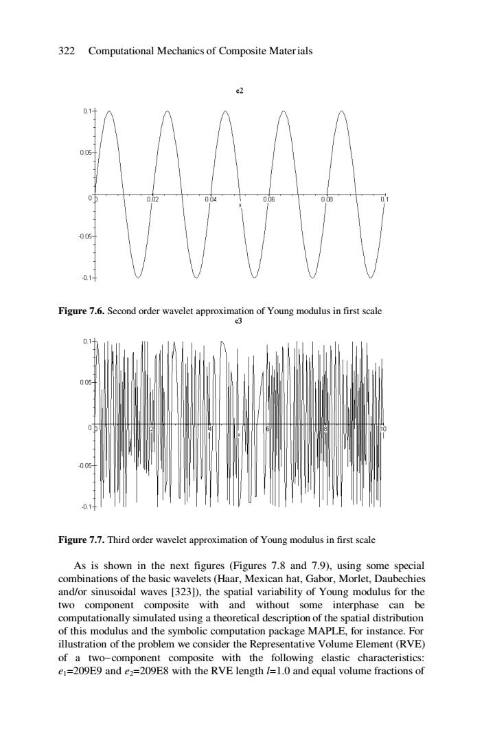
322 Computational Mechanics of Composite Materials e2 0.1+ 0.05 01 0.02 0.04 0.06 008 005 -0.1+ Figure 7.6.Second order wavelet approximation of Young modulus in first scale e3 0.1 0.0吃 0.05 -0.1 Figure 7.7.Third order wavelet approximation of Young modulus in first scale As is shown in the next figures (Figures 7.8 and 7.9),using some special combinations of the basic wavelets (Haar,Mexican hat,Gabor,Morlet,Daubechies and/or sinusoidal waves [323]),the spatial variability of Young modulus for the two component composite with and without some interphase can be computationally simulated using a theoretical description of the spatial distribution of this modulus and the symbolic computation package MAPLE,for instance.For illustration of the problem we consider the Representative Volume Element(RVE) of a two-component composite with the following elastic characteristics: e1=209E9 and e2=209E8 with the RVE length /=1.0 and equal volume fractions of322 Computational Mechanics of Composite Materials Figure 7.6. Second order wavelet approximation of Young modulus in first scale Figure 7.7. Third order wavelet approximation of Young modulus in first scale As is shown in the next figures (Figures 7.8 and 7.9), using some special combinations of the basic wavelets (Haar, Mexican hat, Gabor, Morlet, Daubechies and/or sinusoidal waves [323]), the spatial variability of Young modulus for the two component composite with and without some interphase can be computationally simulated using a theoretical description of the spatial distribution of this modulus and the symbolic computation package MAPLE, for instance. For illustration of the problem we consider the Representative Volume Element (RVE) of a two-component composite with the following elastic characteristics: e1=209E9 and e2=209E8 with the RVE length l=1.0 and equal volume fractions of