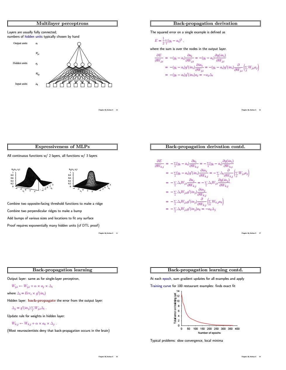
Multilayer perceptrons Back-propagation derivation The squaredsingle example is defined as nb hand E-i-a) =-(ai)g(ini)aj=-ajAi 66占名凸ù Expressiveness of MLPs Back-propagation derivation contd. s w/2 byers,all functions w/3 layers -- 9A Combine tw threshod functions 。-字A,a Combine two perpendicular ridges to make a bump =-AWmm many hidden units (cf DTLproof) Back-propagation learning Back-propagation learning contd. Output layer mes for single-ayer W:-+axa1x△ Training curve for 10 restaurantxmples:findsxfit where△：=Em:xgml iden layer back-propagate from △，=9(m,)ΣWA W一W+a×g×△ (Most deny thaback-proptionin the bain) 5010.15020 203035000 ence.local minim Multilayer perceptrons Layers are usually fully connected; numbers of hidden units typically chosen by hand Input units Hidden units Output units ai Wj,i aj Wk,j ak Chapter 20, Section 5 13 Expressiveness of MLPs All continuous functions w/ 2 layers, all functions w/ 3 layers -4 -2 0 2 x1 4 -4 -2 0 2 4 x2 0 0.2 0.4 0.6 0.8 1 hW (x1 , x2 ) -4 -2 0 2 x1 4 -4 -2 0 2 4 x2 0 0.2 0.4 0.6 0.8 1 hW (x1 , x2 ) Combine two opposite-facing threshold functions to make a ridge Combine two perpendicular ridges to make a bump Add bumps of various sizes and locations to fit any surface Proof requires exponentially many hidden units (cf DTL proof) Chapter 20, Section 5 14 Back-propagation learning Output layer: same as for single-layer perceptron, Wj,i ← Wj,i + α × aj × ∆i where ∆i = Err i × g 0 (ini) Hidden layer: back-propagate the error from the output layer: ∆j = g 0 (inj) X i Wj,i∆i . Update rule for weights in hidden layer: Wk,j ← Wk,j + α × ak × ∆j . (Most neuroscientists deny that back-propagation occurs in the brain) Chapter 20, Section 5 15 Back-propagation derivation The squared error on a single example is defined as E = 1 2 X i (yi − ai) 2 , where the sum is over the nodes in the output layer. ∂E ∂Wj,i = −(yi − ai) ∂ai ∂Wj,i = −(yi − ai) ∂g(ini) ∂Wj,i = −(yi − ai)g 0 (ini) ∂ini ∂Wj,i = −(yi − ai)g 0 (ini) ∂ ∂Wj,i   X j Wj,iaj   = −(yi − ai)g 0 (ini)aj = −aj∆i Chapter 20, Section 5 16 Back-propagation derivation contd. ∂E ∂Wk,j = − X i (yi − ai) ∂ai ∂Wk,j = − X i (yi − ai) ∂g(ini) ∂Wk,j = − X i (yi − ai)g 0 (ini) ∂ini ∂Wk,j = − X i ∆i ∂ ∂Wk,j   X j Wj,iaj   = − X i ∆iWj,i ∂aj ∂Wk,j = − X i ∆iWj,i ∂g(inj ) ∂Wk,j = − X i ∆iWj,ig 0 (inj) ∂inj ∂Wk,j = − X i ∆iWj,ig 0 (inj) ∂ ∂Wk,j   X k Wk,jak   = − X i ∆iWj,ig 0 (inj)ak = −ak∆j Chapter 20, Section 5 17 Back-propagation learning contd. At each epoch, sum gradient updates for all examples and apply Training curve for 100 restaurant examples: finds exact fit 0 2 4 6 8 10 12 14 0 50 100 150 200 250 300 350 400 Total error on training set Number of epochs Typical problems: slow convergence, local minima Chapter 20, Section 5 18