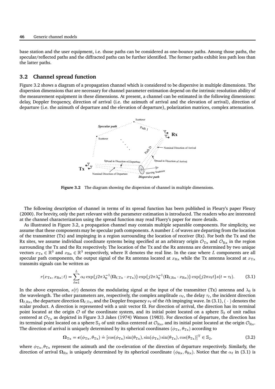
46 Generic channel models the latter paths. 3.2 Channel spread function the measurement equipment in these dimensions.At present,a channel can be estimated in the following dimensions tion or departure. R Figure 3.2 The diagram showing the dispersion of channel in multiple dimensions. The following descipion of hhas been published in Fleury's paper vity,ony the part relevant with e parame d.The reta methat the mponents may be specular path comp A numb or waves a Rx sites,we assume individual coordinate sy tems being specified at an arbitrary origin andO in the region transmits signals can be written as r红，)=oexpfj22r'(xT}ep02=6'(nLxu》epi2mtst-r小 (3.1) n the v()denoe the( the departu direct and the Doppler frequenc of the th impinging In(3.1),(.denotes the A direction is represe ented with a unit vector or direct ction h its nin d as depicted in Pigure 3.3Jakes(197)Watson(19).For direction of departure,the direction has uletely deteninsr rt d on a sphere S2 of uni cated at the origin ORx Srx =e(Tx,Orx)=[cos(orx)sin(0rx),sin(orx)sin(0Tx).cos(0rx)IT ES2. (3.2) 46 Generic channel models base station and the user equipment, i.e. those paths can be considered as one-bounce paths. Among those paths, the specular/reflected paths and the diffracted paths can be further identified. The former paths exhibit less path loss than the latter paths. 3.2 Channel spread function Figure 3.2 shows a diagram of a propagation channel which is considered to be dispersive in multiple dimensions. The dispersion dimensions that are necessary for channel parameter estimation depend on the intrinsic resolution ability of the measurement equipment in these dimensions. At present, a channel can be estimated in the following dimensions: delay, Doppler frequency, direction of arrival (i.e. the azimuth of arrival and the elevation of arrival), direction of departure (i.e. the azimuth of departure and the elevation of departure), polarization matrices, complex attenuation. Tx Moving Scatterer Path 1 Path D Nominal Direction of Departure Nominal Direction of Arrival Rx Scatterer Scatterer Spread in Direction of Departure Spread in Direction of Arrival Specular path Dispersive path Figure 3.2 The diagram showing the dispersion of channel in multiple dimensions. The following description of channel in terms of its spread function has been published in Fleury’s paper Fleury (2000). For brevity, only the part relevant with the parameter estimation is introduced. The readers who are interested at the channel characterization using the spread function may read Fluery’s paper for more details. As illustrated in Figure 3.2, a propagation channel may contain multiple separable components. For simplicity, we assume that these components may be specular path components. A number L of waves are departing from the location of the transmitter (Tx) and impinging in a region surrounding the location of receiver (Rx). For both the Tx and the Rx sites, we assume individual coordinate systems being specified at an arbitrary origin OTx and ORx in the region surrounding the Tx and the Rx respectively. The location of the Tx and the Rx antenna are determined by two unique vectors xTx ∈ R 3 and xRx ∈ R 3 respectively, where R denotes the real line. In the case where L components are all specular path components, the output signal of the Rx antenna located at xRx while the Tx antenna located at xTx transmits signals can be written as r(xTx, xRx;t) = X L ℓ=1 αℓ exp{j2πλ−1 0 (Ωℓ,Tx · xTx)} exp{j2πλ−1 0 (Ωℓ,Rx · xRx)} exp{j2πνℓt}s(t − τℓ). (3.1) In the above expression, s(t) denotes the modulating signal at the input of the transmitter (Tx) antenna and λ0 is the wavelength. The other parameters are, respectively, the complex amplitude αℓ, the delay τℓ, the incident direction Ωℓ,Rx, the departure direction Ωℓ,Tx, and the Doppler frequency νℓ of the ℓth impinging wave. In (3.1), ( · ) denotes the scalar product. A direction is represented with a unit vector Ω. For direction of arrival, the direction has its terminal point located at the origin O of the coordinate system, and its initial point located on a sphere S2 of unit radius centered at OTx as depicted in Figure 3.3 Jakes (1974) Watson (1983). For direction of departure, the direction has its terminal point located on a sphere S2 of unit radius centered at ORx, and its initial point located at the origin ORx. The direction of arrival is uniquely determined by its spherical coordinates (φTx, θTx) according to ΩTx = e(φTx, θTx) .= [cos(φTx) sin(θTx),sin(φTx) sin(θTx), cos(θTx)]T ∈ S2, (3.2) where φTx, θTx represent the azimuth and the co-elevation of the direction of departure respectively. Similarly, the direction of arrival ΩRx is uniquely determined by its spherical coordinate (φRx, θRx). Notice that the αℓ in (3.1) is