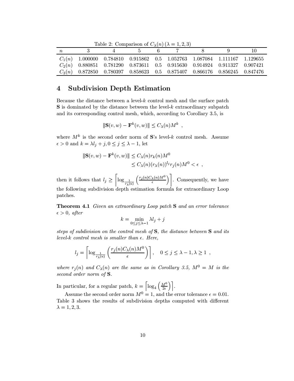
Table 2:Comparison of C(m)(12.3) 88的照e 4 Subdivision Depth Estimation Ise,回-Pe,sCma A光a0空m.e ISe,回)-e,训sCrx ≤((,<t a1Cmenmaya8almmrnm k=,M+方 10 Table 2: Comparison of Cλ(n) (λ = 1, 2, 3) n 3 4 5 6 7 8 9 10 C1(n) 1.000000 0.784810 0.915862 0.5 1.052763 1.087084 1.111167 1.129655 C2(n) 0.880851 0.781290 0.873611 0.5 0.915630 0.914924 0.911327 0.907421 C3(n) 0.872850 0.780397 0.858623 0.5 0.875407 0.866176 0.856245 0.847476 4 Subdivision Depth Estimation Because the distance between a level-k control mesh and the surface patch S is dominated by the distance between the level-k extraordinary subpatch and its corresponding control mesh, which, according to Corollary 3.5, is kS(v, w) − F k (v, w)k ≤ Cλ(n)Mk , where Mk is the second order norm of S’s level-k control mesh. Assume ǫ > 0 and k = λlj + j, 0 ≤ j ≤ λ − 1, let kS(v, w) − F k (v, w)k ≤ Cλ(n)rk(n)M0 ≤ Cλ(n)(rλ(n))lj rj (n)M0 < ǫ , then it follows that lj ≥  log 1 rλ(n)  rj (n)Cλ(n)M0 ǫ  . Consequently, we have the following subdivision depth estimation formula for extraordinary Loop patches. Theorem 4.1 Given an extraordinary Loop patch S and an error tolerance ǫ > 0, after k = min 0≤j≤λ−1 λlj + j steps of subdivision on the control mesh of S, the distance between S and its level-k control mesh is smaller than ǫ. Here, lj =  log 1 rλ(n)  rj (n)Cλ(n)M0 ǫ  , 0 ≤ j ≤ λ − 1, λ ≥ 1 , where rj (n) and Cλ(n) are the same as in Corollary 3.5, M0 = M is the second order norm of S. In particular, for a regular patch, k = l log4  M0 2ǫ m. Assume the second order norm M0 = 1, and the error tolerance ǫ = 0.01. Table 3 shows the results of subdivision depths computed with different λ = 1, 2, 3. 10