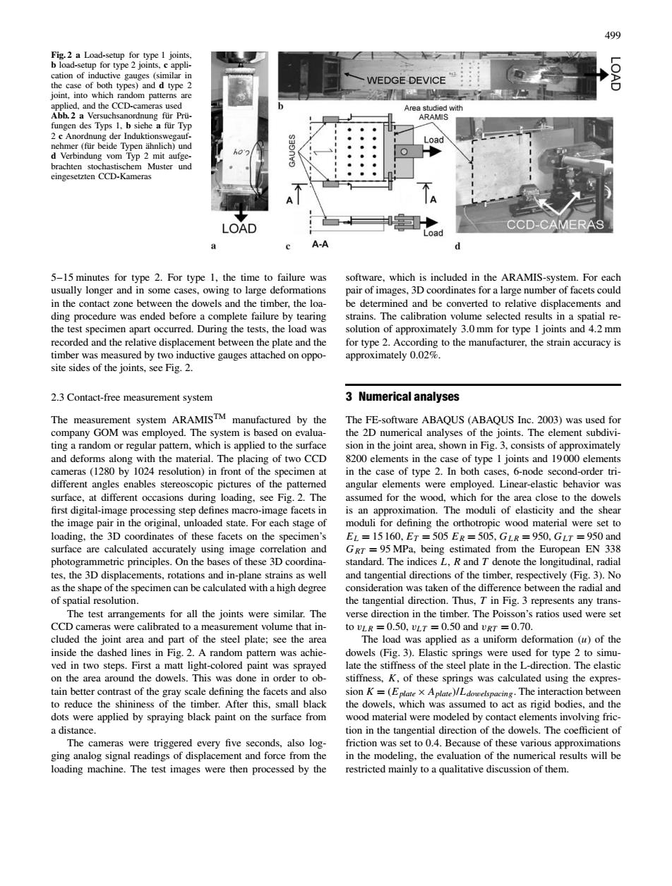
499 Load en CCD-Kae LOAD CCDECAME which is incuded in the ARAMIS-ystem For eac in the contact zone hetween the dowels and the timber the lo be determined and be converted to relative displacements and strains.The calibration volume selected results ed. the tes approximately 3.0mm for type was measured by two inductive gauges attached on oppo site sides of the joints.see Fig.2. 2.3 Contact-free measurement system 3 Numerical analyses ARAMISTM ABAQUS In 20wsus for ting a random or regular pattem.which is applied to the surfac sion in the joint area.shown in Fig.3.consists of apr oximately and deform ment red.Linear-elastic pehavior was surface.at different occasions during loading.see Fig.2.The assumed for the wood,which for the area close to the dowels air in th mag y loading.the 3D coordinates of these facets on the specim en's EL=15160.E7=505ER=505.G1R=950.GL7=950an lation and 3D GT=5 MPa. al dire s of the N ig. imila Th any tran =0.50.7=0.50 and var=0.70 luded the joint area and part of the stel plate;see the he load vas applied as a uniform deformation (of the was achi the on the area around the dowels.This was done in order to o stiffness.K.of these springs was calculated using the expres ain better ast of the gray sca ung the facets and =(E The in dots were applied by spraying black paint on the surface from d material were e modeled by contact elements involving fric a distance ion in the tangential direction of the dowels.The coefficient of also log on was set te nd fo restricted mainly to a qualitative discussion of them. 499 Fig. 2 a Load-setup for type 1 joints, b load-setup for type 2 joints, c appli￾cation of inductive gauges (similar in the case of both types) and d type 2 joint, into which random patterns are applied, and the CCD-cameras used Abb. 2 a Versuchsanordnung für Prü- fungen des Typs 1, b siehe a für Typ 2 c Anordnung der Induktionswegauf￾nehmer (für beide Typen ähnlich) und d Verbindung vom Typ 2 mit aufge￾brachten stochastischem Muster und eingesetzten CCD-Kameras 5–15 minutes for type 2. For type 1, the time to failure was usually longer and in some cases, owing to large deformations in the contact zone between the dowels and the timber, the loa￾ding procedure was ended before a complete failure by tearing the test specimen apart occurred. During the tests, the load was recorded and the relative displacement between the plate and the timber was measured by two inductive gauges attached on oppo￾site sides of the joints, see Fig. 2. 2.3 Contact-free measurement system The measurement system ARAMISTM manufactured by the company GOM was employed. The system is based on evalua￾ting a random or regular pattern, which is applied to the surface and deforms along with the material. The placing of two CCD cameras (1280 by 1024 resolution) in front of the specimen at different angles enables stereoscopic pictures of the patterned surface, at different occasions during loading, see Fig. 2. The first digital-image processing step defines macro-image facets in the image pair in the original, unloaded state. For each stage of loading, the 3D coordinates of these facets on the specimen’s surface are calculated accurately using image correlation and photogrammetric principles. On the bases of these 3D coordina￾tes, the 3D displacements, rotations and in-plane strains as well as the shape of the specimen can be calculated with a high degree of spatial resolution. The test arrangements for all the joints were similar. The CCD cameras were calibrated to a measurement volume that in￾cluded the joint area and part of the steel plate; see the area inside the dashed lines in Fig. 2. A random pattern was achie￾ved in two steps. First a matt light-colored paint was sprayed on the area around the dowels. This was done in order to ob￾tain better contrast of the gray scale defining the facets and also to reduce the shininess of the timber. After this, small black dots were applied by spraying black paint on the surface from a distance. The cameras were triggered every five seconds, also log￾ging analog signal readings of displacement and force from the loading machine. The test images were then processed by the software, which is included in the ARAMIS-system. For each pair of images, 3D coordinates for a large number of facets could be determined and be converted to relative displacements and strains. The calibration volume selected results in a spatial re￾solution of approximately 3.0 mm for type 1 joints and 4.2 mm for type 2. According to the manufacturer, the strain accuracy is approximately 0.02%. 3 Numerical analyses The FE-software ABAQUS (ABAQUS Inc. 2003) was used for the 2D numerical analyses of the joints. The element subdivi￾sion in the joint area, shown in Fig. 3, consists of approximately 8200 elements in the case of type 1 joints and 19 000 elements in the case of type 2. In both cases, 6-node second-order tri￾angular elements were employed. Linear-elastic behavior was assumed for the wood, which for the area close to the dowels is an approximation. The moduli of elasticity and the shear moduli for defining the orthotropic wood material were set to EL = 15 160, ET = 505 ER = 505, GL R = 950, GLT = 950 and GRT = 95 MPa, being estimated from the European EN 338 standard. The indices L, R and T denote the longitudinal, radial and tangential directions of the timber, respectively (Fig. 3). No consideration was taken of the difference between the radial and the tangential direction. Thus, T in Fig. 3 represents any trans￾verse direction in the timber. The Poisson’s ratios used were set to vL R = 0.50, vLT = 0.50 and vRT = 0.70. The load was applied as a uniform deformation (u) of the dowels (Fig. 3). Elastic springs were used for type 2 to simu￾late the stiffness of the steel plate in the L-direction. The elastic stiffness, K, of these springs was calculated using the expres￾sion K = (Eplate × Aplate)/Ldowelspacing. The interaction between the dowels, which was assumed to act as rigid bodies, and the wood material were modeled by contact elements involving fric￾tion in the tangential direction of the dowels. The coefficient of friction was set to 0.4. Because of these various approximations in the modeling, the evaluation of the numerical results will be restricted mainly to a qualitative discussion of them