1 Mathematical Preliminaries 1.1 Probability Theory Elements 1.1.1 Introduction Probability theory [326,357,365]is a part of theoretical and applied mathematics, which is engaged in establishing the rules governing random events-random games or experimental testing.The definitions,theorems and lemmas given below are necessary to understand the basic equations and computer implementation aspects used in the later numerical analyses presented in the book.They can also be used to calculate many of the closed-form equations applied frequently in applied sciences and engineering practice [19,37,150,201,202,253]. Definition The variations with n elements for k elements are k elements series where each number 1,2,...k corresponds to the single element from the initial set.The variations can differ in the elements or their order.The total number of all variations with n elements for k is described by the relation (n-k):=nn-D..(n-k+1) n! (1.1) k-times Example Let us consider the three-element set A(X,Y,Z).Two-element variations of this set are represented as V2=6:XY,YZ,XZ,YX,ZY,ZX. Definition Permutations with n elements are n-element series where each number 1,2,...,n corresponds to the single element from the initial n-element set.The difference between permutations is in the element order.The total number of all permutations with n different elements is given by the formula: Pn=V=1.2…n=nl (1.2) If among n elements X,Y,Z....there are identical elements,where X repeats a times,Y appears b times,while Z repeats c times etc.,then
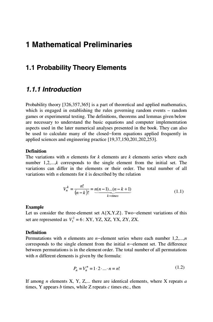
1 Mathematical Preliminaries 1.1 Probability Theory Elements 1.1.1 Introduction Probability theory [326,357,365] is a part of theoretical and applied mathematics, which is engaged in establishing the rules governing random events – random games or experimental testing. The definitions, theorems and lemmas given below are necessary to understand the basic equations and computer implementation aspects used in the later numerical analyses presented in the book. They can also be used to calculate many of the closed-form equations applied frequently in applied sciences and engineering practice [19,37,150,201,202,253]. Definition The variations with n elements for k elements are k elements series where each number 1,2,...,k corresponds to the single element from the initial set. The variations can differ in the elements or their order. The total number of all variations with n elements for k is described by the relation ( ) 14 2 44 4 3 44 k times k n n n n k n k n V − = − − + − = ( 1)...( 1) ! ! (1.1) Example Let us consider the three-element set A{X,Y,Z}. Two-element variations of this set are represented as 6 2 V3 = : XY, YZ, XZ, YX, ZY, ZX. Definition Permutations with n elements are n-element series where each number 1,2,...,n corresponds to the single element from the initial n-element set. The difference between permutations is in the element order. The total number of all permutations with n different elements is given by the formula: P V 1 2 ... n n! n n = n = ⋅ ⋅ ⋅ = (1.2) If among n elements X, Y, Z,... there are identical elements, where X repeats a times, Y appears b times, while Z repeats c times etc., then
2 Computational Mechanics of Composite Materials (1.3) alblc! Example Let us consider the three element set A[X,Y,Z).The following permutations of the set A are available:P=6:XYZ,XZY,YZX,YXZ,ZXY,ZYX. Definition The combinations with n elements for k elements are k-elements sets,which can be created by choosing any k elements from the given n-element set,where the order does not play any role.The combinations can differ in the elements only.The total number of all combinations with n for k elements is described by the formula k(n-k)月 (1.4) In specific cases it is found that c0c- (1.5) where G (1.6) Example Let us consider a set AfX,Y,Z)as before.Two-element variations of this set are the following:XY,XZ and YZ. The fundamental concepts of probability theory are random experiments and random events resulting from them.A single event,which can result from some random experiment is called elementary event,an and for the single die throw is equivalent to any sum of the dots on a die taken from the set {1,...,6).Further,it is concluded that all elementary events corresponding to the random experiment form the elementary events space defined usually as which various subsets like A and/or B belong to (favouring the specified event or not,for instance). Definition A formal notation A denotes that the elementary event co belongs to the event A and is understood in the following way-if c results from some experiment,then the event A happened too,which c belongs to.The notation means that the elementary event c favours the event A
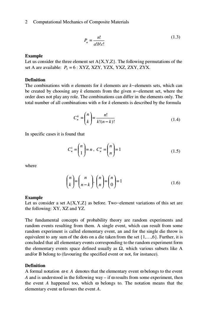
2 Computational Mechanics of Composite Materials ! ! ! ! a b c n Pn = (1.3) Example Let us consider the three element set A{X,Y,Z}. The following permutations of the set A are available: 6 P3 = : XYZ, XZY, YZX, YXZ, ZXY, ZYX. Definition The combinations with n elements for k elements are k-elements sets, which can be created by choosing any k elements from the given n-element set, where the order does not play any role. The combinations can differ in the elements only. The total number of all combinations with n for k elements is described by the formula !( )! ! k n k n k n Ck n − =⎟ ⎟ ⎠ ⎞ ⎜ ⎜ ⎝ ⎛ = (1.4) In specific cases it is found that n n Cn =⎟ ⎟ ⎠ ⎞ ⎜ ⎜ ⎝ ⎛ = 1 1 , 1 =⎟ ⎟ ⎠ ⎞ ⎜ ⎜ ⎝ ⎛ = n n Cn n (1.5) where ⎟ ⎟ ⎠ ⎞ ⎜ ⎜ ⎝ ⎛ − =⎟ ⎟ ⎠ ⎞ ⎜ ⎜ ⎝ ⎛ n k n k n , 1 0 =⎟ ⎟ ⎠ ⎞ ⎜ ⎜ ⎝ ⎛ =⎟ ⎟ ⎠ ⎞ ⎜ ⎜ ⎝ ⎛ n n n (1.6) Example Let us consider a set A{X,Y,Z} as before. Two-element variations of this set are the following: XY, XZ and YZ. The fundamental concepts of probability theory are random experiments and random events resulting from them. A single event, which can result from some random experiment is called elementary event, an and for the single die throw is equivalent to any sum of the dots on a die taken from the set {1,…,6}. Further, it is concluded that all elementary events corresponding to the random experiment form the elementary events space defined usually as Ω, which various subsets like A and/or B belong to (favouring the specified event or not, for instance). Definition A formal notation ω ∈ A denotes that the elementary event ω belongs to the event A and is understood in the following way – if ω results from some experiment, then the event A happened too, which ω belongs to. The notation means that the elementary event ω favours the event A
Mathematical Preliminaries 3 Definition The formal notation Ac B,which means that event A is included in the event B is understood such that event A results in the event B since the following implication holds true:if the elementary event co favours event A,then event o favours event B,too. Definition An alternative of the events A.A......A is the following sum: A 0A 0...0A =UA (1.7) which is a random event consisting of all random elementary events belonging to at least one of the events A,A2,....A. Definition A conjunction of the events A,A2,....A is a product A∩A2∩.nAn=∩A (1.8) which proceeds if and only if any of the events A,A.,...,A proceed Definition Probability is a function P which is defined on the subsets of the elementary events and having real values in closed interval [0,1]such that (1)P(2)=1,P(0)=0: (2)for any finite and/or infinite series of the excluding events A,A2,...A,... A,A,=☑,there holds for itj AFΣPA) (1.9) Starting from the above definitions one can demonstrate the following lemmas: Lemma The probability of the alternative of the events is equal to the sum of the probabilities of these events. Lemma If event B results from event A then
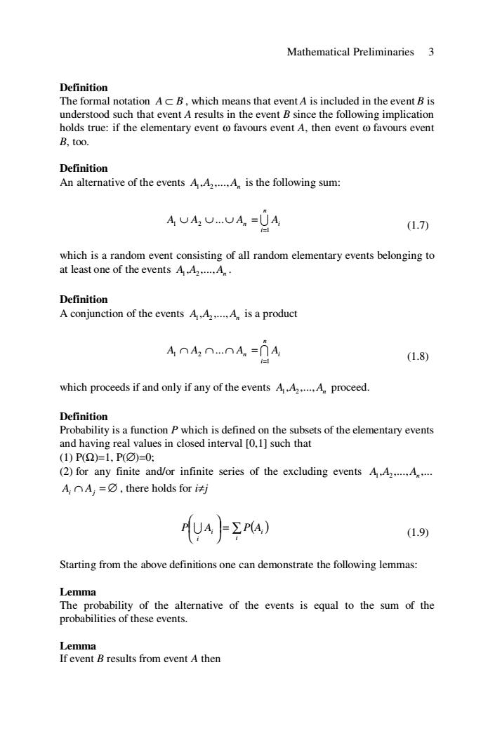
Mathematical Preliminaries 3 Definition The formal notation A ⊂ B , which means that event A is included in the event B is understood such that event A results in the event B since the following implication holds true: if the elementary event ω favours event A, then event ω favours event B, too. Definition An alternative of the events A A An , ,..., 1 2 is the following sum: U n i A A An Ai 1 1 2 ... = ∪ ∪ ∪ = (1.7) which is a random event consisting of all random elementary events belonging to at least one of the events A A An , ,..., 1 2 . Definition A conjunction of the events A A An , ,..., 1 2 is a product I n i A A An Ai 1 1 2 ... = ∩ ∩ ∩ = (1.8) which proceeds if and only if any of the events A A An , ,..., 1 2 proceed. Definition Probability is a function P which is defined on the subsets of the elementary events and having real values in closed interval [0,1] such that (1) P(Ω)=1, P(∅)=0; (2) for any finite and/or infinite series of the excluding events ,... , ,..., A1 A2 An Ai ∩ Aj = ∅ , there holds for i≠j ⎟ = ∑ ( ) ⎠ ⎞ ⎜ ⎝ ⎛ i i i P UAi P A (1.9) Starting from the above definitions one can demonstrate the following lemmas: Lemma The probability of the alternative of the events is equal to the sum of the probabilities of these events. Lemma If event B results from event A then
4 Computational Mechanics of Composite Materials P(A)<P(B) (1.10) The definition of probability does not reflect however a natural very practical need of its value determination and that is why the simplified Laplace definition is frequently used for various random events. Definition If n trials forms the random space of elementary events where each experiment has the same probability equal to 1/n,then the probability of the m-element event A is equal to P(A)= (1.11) Next,we will explain the definition,meaning and basic properties of the probability spaces.The probability space(,F,P)is uniquely defined by the space of elementary random events the events field F and probabilistic measure P. The field of events F is the relevant family of subsets of the space of elementary random events This field F is a non-empty,complementary and countable additive set having o-algebra structure. Definition The probabilistic measure P is a function P:F→[0,] (1.12) which is a nonnegative,countable additive and normalized function defined on the fields of random events.The pair (F)is a countable space,while the events are countable subsets of The value P(A)assigned by the probabilistic measure P to event A is called a probability of this event. Definition Two events A and B are independent if they fulfil the following condition: P(AOB)=P(A)P(B) (1.13) while the events A.AA are pair independent,if this condition holds true for any pair from this set. Definition Let us consider the probability space (.F.P)and measurable spaceB. where B is a class of the Borelian sets.Then,the representation
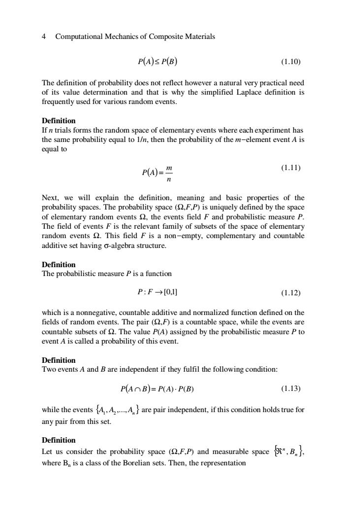
4 Computational Mechanics of Composite Materials P() () A ≤ P B (1.10) The definition of probability does not reflect however a natural very practical need of its value determination and that is why the simplified Laplace definition is frequently used for various random events. Definition If n trials forms the random space of elementary events where each experiment has the same probability equal to 1/n, then the probability of the m-element event A is equal to ( ) n m P A = (1.11) Next, we will explain the definition, meaning and basic properties of the probability spaces. The probability space (Ω,F,P) is uniquely defined by the space of elementary random events Ω, the events field F and probabilistic measure P. The field of events F is the relevant family of subsets of the space of elementary random events Ω. This field F is a non-empty, complementary and countable additive set having σ-algebra structure. Definition The probabilistic measure P is a function P : F →[0,1] (1.12) which is a nonnegative, countable additive and normalized function defined on the fields of random events. The pair (Ω,F) is a countable space, while the events are countable subsets of Ω. The value P(A) assigned by the probabilistic measure P to event A is called a probability of this event. Definition Two events A and B are independent if they fulfil the following condition: P( ) A∩ B = P(A)⋅ P(B) (1.13) while the events { } A A An , ,..., 1 2 are pair independent, if this condition holds true for any pair from this set. Definition Let us consider the probability space (Ω,F,P) and measurable space { }n n ℜ , B , where Bn is a class of the Borelian sets. Then, the representation
Mathematical Preliminaries 5 X:2→R” (1.14) is an n-dimensional random variable or n-dimensional random vector. Definition The probability distribution of the random variable X is a function Px:B[0,1] such that Px(b)=P(X∈B) (1.15) be B The probability distribution of the random variable is a probabilistic measure. Definition Let us consider the following probability space (,B,Px).The function Fx:gr→[0,1]defined as F(x)=Px《-∞,xl (1.16) is called the cumulative distribution function of the variable X. Definition The function f:,has the following properties: (1)there holds almost everywhere (in each point of the cumulative distribution function differentiability): dF(x)=f(x) (1.17) dx (2) f(x)20 (1.18) (3) Jrcod=1 (1.19) (4)for any Borelian set beB the integral ff(x)dx=P(Xeb)is a probability density function(PDF)of the variable X. Definition Let us consider the random variable X:defined on the probabilistic space (F,P).The expected value of the random variable X is defined as EX]=∫X(o)dP(o) (1.20)
Mathematical Preliminaries 5 n X :Ω → ℜ (1.14) is an n-dimensional random variable or n-dimensional random vector. Definition The probability distribution of the random variable X is a function ] P : B →[0,1 X such that P (b) P(X B) X b B ∀ = ∈ ∈ (1.15) The probability distribution of the random variable is a probabilistic measure. Definition Let us consider the following probability space ( ) B PX ℜ, , . The function :ℜ →[0,1] FX defined as F x P [ ] ( ) x X ( ) = − ∞, (1.16) is called the cumulative distribution function of the variable X. Definition The function ℜ → ℜ+ f : has the following properties: (1) there holds almost everywhere (in each point of the cumulative distribution function differentiability): ( ) ( ) f x dx dF x = (1.17) (2) f (x) ≥ 0 (1.18) (3) ∫ +∞ −∞ f (x)dx = 1 (1.19) (4) for any Borelian set b ∈ B the integral ( ) ∫ = ∈ b f ( is a probability x)dx P X b density function (PDF) of the variable X. Definition Let us consider the random variable X :Ω → ℜ defined on the probabilistic space ( ) Ω, F, P . The expected value of the random variable X is defined as ∫ +∞ −∞ E[X ] = X (ω)dP(ω) (1.20)
6 Computational Mechanics of Composite Materials if only the Lesbegue integral with respect to the probabilistic measure exists and converges. Lemma Eel=e (1.21) Lemma There holds for any random numbers X and the real numbers c,E (1.22) Lemma There holds for any independent random variables X ex.-fex.] (1.23) Definition Let us consider the following random variable X:defined on the probabilistic space (F,P).The variance of the variable X is defined as Var(X)=[(X(@)-E[X]YdP(@) (1.24) Q and the standard deviation is called the quantity G(X)=Var(X) (1.25) Lemma 女Var(c)=0 (1.26 Lemma Y Var(cX)=c-Var(X) (1.27) E Lemma There holds for any two independent random variables X and Y Var(X +Y)=Var(X)+Var(Y) (1.28) Var(X.Y)=E[X].Var(Y)+Var(X).Var(Y)+Var(X).E[Y] (1.29)
6 Computational Mechanics of Composite Materials if only the Lesbegue integral with respect to the probabilistic measure exists and converges. Lemma E c c c ∀ = ∈ℜ [ ] (1.21) Lemma There holds for any random numbers Xi and the real numbers ci ∈ℜ ∑ ∑ [ ] = = =⎥ ⎦ ⎤ ⎢ ⎣ ⎡ n i i i n i E ci Xi c E X 1 1 (1.22) Lemma There holds for any independent random variables Xi ∏ ∏ [ ] = ⎥ = ⎦ ⎤ ⎢ ⎣ ⎡ = n i i n i E X i E X 1 1 (1.23) Definition Let us consider the following random variable X :Ω → ℜ defined on the probabilistic space ( ) Ω, F, P . The variance of the variable X is defined as ( ) [ ] ∫ Ω ( ) = ( ) − ( ) 2 Var X X ω E X dP ω (1.24) and the standard deviation is called the quantity σ (X) = Var(X ) (1.25) Lemma ∀ ( ) = 0 ∈ℜ Var c c (1.26) Lemma ( ) ( ) 2 Var cX c Var X c ∀ = ∈ℜ (1.27) Lemma There holds for any two independent random variables X and Y Var( ) X ± Y = Var(X) +Var(Y) (1.28) ( ) [ ] ( ) ( ) ( ) ( ) [ ] 2 2 Var X ⋅Y = E X ⋅Var Y +Var X ⋅Var Y +Var X ⋅ E Y (1.29)
Mathematical Preliminaries 7 Definition Let us consider the random variable X:defined on the probabilistic space (2,F,P).A complex function of the real variable o:Z such that p(t)=Eexp(itx】 (1.30) stands for the characteristic function of the variable X. 1.1.2 Gaussian and Quasi-Gaussian Random Variables Let us consider the random variable X having a Gaussian probability distribution function with m being the expected value and o >0 the standard deviation.The distribution function of this variable is (1.31) where the probability density function is calculated as f)= exp (r-m)2 202 (1.32) The characteristic function for this variable is denoted as o(t)=Elexp(itx)]=exp(mit-2). (1.33) If the variable X with the parameters(m,o)is Gaussian,then its linear transform Y=AX +B with A,Be is Gaussian,too,and its parameters are equal to Am+B and Ao for A≠0,respectively. Problem Let us consider the random variable X with the first two moments E[X]and Var(X). Let us determine the corresponding moments of the new variable Y=X2. Solution The problem has been solved using three different ways illustrating various methods applicable in this and in analogous cases.The generality of these methods make them available in the determination of probabilistic moments and their parameters for most random variables and their transforms for given or unknown
Mathematical Preliminaries 7 Definition Let us consider the random variable X :Ω → ℜ defined on the probabilistic space ( ) Ω, F, P . A complex function of the real variable ϕ :ℜ → Z such that ϕ(t) = E[ ] exp(itX ) (1.30) stands for the characteristic function of the variable X. 1.1.2 Gaussian and Quasi-Gaussian Random Variables Let us consider the random variable X having a Gaussian probability distribution function with m being the expected value and 0 σ > the standard deviation. The distribution function of this variable is dt t F x x ∫ −∞ ⎟ ⎟ ⎠ ⎞ ⎜ ⎜ ⎝ ⎛ − = 2 exp 2 1 ( ) 2 π (1.31) where the probability density function is calculated as ⎟ ⎟ ⎠ ⎞ ⎜ ⎜ ⎝ ⎛ − = − 2 2 2 ( ) exp 2 1 ( ) σ π σ x m f x (1.32) The characteristic function for this variable is denoted as [ ] ( ) 2 2 2 1 ϕ(t) = E exp(itX ) = exp mit − σ t . (1.33) If the variable X with the parameters (m,σ) is Gaussian, then its linear transform Y = AX + B with A, is Gaussian, too, and its parameters are equal to B ∈ℜ Am+B and Aσ for 0 A ≠ , respectively. Problem Let us consider the random variable X with the first two moments E[X] and Var(X). Let us determine the corresponding moments of the new variable 2 Y = X . Solution The problem has been solved using three different ways illustrating various methods applicable in this and in analogous cases. The generality of these methods make them available in the determination of probabilistic moments and their parameters for most random variables and their transforms for given or unknown
8 Computational Mechanics of Composite Materials probability density functions of the input frequently takes place in which numerous engineering problems. I method Starting from the definition of the variance of a ny random variable one can write Var(Y)=E(Y2)-E2(Y) (1.34) Let Y=X2,then Var(X2)=E(X2)2)-E2(X2) (1.35) The value of E will be determined through integration of the characteristic function for the Gaussian probability density function (1.36) where m=E[X]and o=Var(X)denote the expected value and standard deviation of the considered distribution,respectively.Next,the following standardised variable is introduced t=x-m,where x=to+m,dx=adt (1.37) which gives k了+mreu叫} (1.38) After some algebraic transforms of the integrand function it is obtained that Ek☆了(or+4onmn户+6anm+4omr+me号h (1.39) and,dividing into particular integrals,there holds Ek]应oh+4oml,+6o2m21,+4om14+m1,)e号 (1.40) where the components denote
8 Computational Mechanics of Composite Materials probability density functions of the input frequently takes place in which numerous engineering problems. I method Starting from the definition of the variance of a ny random variable one can write ( ) ( ) ( ) 2 2 Var Y = E Y − E Y (1.34) Let 2 Y = X , then ( ) (( ) ) ( ) 2 2 2 2 2 Var X = E X − E X (1.35) The value of [ ] 4 E X will be determined through integration of the characteristic function for the Gaussian probability density function [ ] ∫ +∞ −∞ ⎟ ⎟ ⎠ ⎞ ⎜ ⎜ ⎝ ⎛ − = − dx x m E X x 2 2 4 2 4 1 2 ( ) exp σ π σ (1.36) where m=E[X] and σ = Var(X ) denote the expected value and standard deviation of the considered distribution, respectively. Next, the following standardised variable is introduced σ x m t − = , where x = tσ + m,dx = σdt (1.37) which gives [ ] dt t E X ∫ t m +∞ −∞ ⎟ ⎟ ⎠ ⎞ ⎜ ⎜ ⎝ ⎛ = + − 2 ( ) exp 2 4 2 4 1 σ π (1.38) After some algebraic transforms of the integrand function it is obtained that E[ ] X t mt m t m t m e dt t ∫ +∞ −∞ − = + + + + 2 2 ( 4 6 4 ) 4 4 3 3 2 2 2 3 4 2 4 1 σ σ σ σ π (1.39) and, dividing into particular integrals, there holds [ ] 2 2 ( 4 6 4 ) 5 4 4 3 3 2 2 2 3 1 4 2 4 1 t E X I mI m I m I m I e − = σ + σ + σ + σ + π (1.40) where the components denote
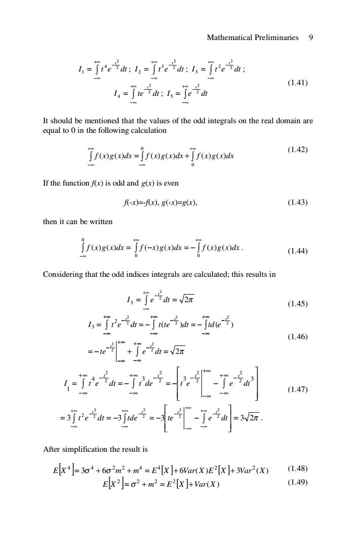
Mathematical Preliminaries 9 1,=jre号d:l,=jre9d;l,=jre号d: (1.41) I=jted:Is=jed It should be mentioned that the values of the odd integrals on the real domain are equal to 0 in the following calculation jf(x)g(x)dx-jf()g(dx+jf(x)g(x)d (1.42) If the function fx)is odd and g(x)is even x)=-fx),g(x)=g(x), (1.43) then it can be written jrd--d--d (1.44) Considering that the odd indices integrals are calculated;this results in 1,=je片di=际 (1.45) 5=rah=-了eh=-de5, (1.46) ∫e d=V2 4a-了-. (1.47) =-a-[-w际 After simplification the result is Ex4]=30+602m2+m=E+[X ]+6Var(X)E2[X]+3Var2(X) (1.48) Ex2=o2+m2=E2[X]+Var(X) (1.49)
Mathematical Preliminaries 9 I t e dt t ∫ +∞ −∞ − = 2 2 4 1 ; I t e dt t ∫ +∞ −∞ − = 2 2 3 2 ; I t e dt t ∫ +∞ −∞ − = 2 2 2 3 ; I te dt t ∫ +∞ −∞ − = 2 2 4 ; I e dt t ∫ +∞ −∞ − = 2 2 5 (1.41) It should be mentioned that the values of the odd integrals on the real domain are equal to 0 in the following calculation ∫ ∫ ∫ +∞ −∞ +∞ −∞ = + 0 0 f (x)g(x)dx f (x)g(x)dx f (x)g(x)dx (1.42) If the function f(x) is odd and g(x) is even f(-x)=-f(x), g(-x)=g(x), (1.43) then it can be written ∫ ∫ ∫ +∞ +∞ −∞ = − = − 0 0 0 f (x)g(x)dx f ( x)g(x)dx f (x)g(x)dx . (1.44) Considering that the odd indices integrals are calculated; this results in 2π 2 2 5 = ∫ = +∞ −∞ − I e dt t (1.45) 2π ( ) ( ) 2 2 2 2 2 2 2 2 2 2 2 3 = − + = = = − = − ∫ ∫ ∫ ∫ +∞ −∞ − +∞ −∞ − − +∞ −∞ +∞ −∞ − +∞ −∞ − te e dt I t e dt t te dt td e t t t t t (1.46) ⎥ ⎥ ⎥ ⎦ ⎤ ⎢ ⎢ ⎢ ⎣ ⎡ = ∫ = − ∫ = − − ∫ +∞ −∞ − +∞ −∞ − − +∞ −∞ +∞ −∞ 4 − 3 3 3 1 2 2 2 2 2 2 2 2 I t e dt t de t e e dt t t t t 3 3 3 3 2π 2 2 2 2 2 2 2 2 2 = ⎥ ⎥ ⎦ ⎤ ⎢ ⎢ ⎣ ⎡ = ∫ = − ∫ = − − ∫ +∞ −∞ − +∞ −∞ − − +∞ −∞ +∞ −∞ − t e dt tde te e dt t t t t . (1.47) After simplification the result is [ ] 3 6 [] [] 6 ( ) 3 ( ) 4 4 2 2 4 4 2 2 E X = σ + σ m + m = E X + Var X E X + Var X (1.48) [ ] [ ] ( ) 2 2 2 2 E X = σ + m = E X +Var X (1.49)

10 Computational Mechanics of Composite Materials Var(x3=E4E2k2=2o2(o2+2m2) (1.50) =2Var(X)(Var(X)+2E2[X) IⅡnethod Initial algebraic rules can be proved following the method shown below.Using a modified algebraic definition of the variance Var(x2)=Ex-E2x*] (1.51) and the expected value Elx2]=Var(X)+E"[x] (1.52) subtracted from the following equation E2x=(Var(X)+E2[x]=Var2x+2Var(X)E2[x]+E[x] (1.53) we can demonstrate the following desired result: Var(X2)=EX-Var2(X)-2Var(X)E2[X]-E[X] (1.54) III method The characteristic function for the Gaussian PDF has the following form: p()=exp(mit--o2r2)】 (1.55) where p(0=*Ex}5k≥0 (1.56 and =(0)=im (1.57) The mathematical induction rule leads us to the conclusion that pm)=m-to2pm-(0-(0n-1o2.pa-2》0),n≥2 (1.58) which results in the equations
10 Computational Mechanics of Composite Materials [ ] [ ] 2 ( )( ( ) 2 [ ]) ( ) 2 ( 2 ) 2 2 4 2 2 2 2 2 Var X Var X E X Var X E X E X m = + = − = σ σ + (1.50) II method Initial algebraic rules can be proved following the method shown below. Using a modified algebraic definition of the variance [] [] 2 4 2 2 Var(X ) = E X − E X (1.51) and the expected value E[X ] Var X E [ ] X 2 2 = ( ) + (1.52) subtracted from the following equation E [ ] X ( ) Var X E [ ] X Var X Var X E [] [] X E X 2 2 4 2 2 2 2 = ( ) + = + 2 ( ) + (1.53) we can demonstrate the following desired result: Var X E[X ] Var X Var X E X E [ ] X 2 4 2 2 4 ( ) = − ( ) − 2 ( ) [ ] − (1.54) III method The characteristic function for the Gaussian PDF has the following form: ( ) 2 2 2 1 ϕ(t) = exp mit − σ t (1.55) where [ ] k k k (0) = i E X ( ) ϕ ; k ≥ 0 (1.56) and ϕ = ϕ (0) ; ϕ′(0) = im (1.57) The mathematical induction rule leads us to the conclusion that ( ) ( ) ( ) ( 1) ( ) ( ) 2 ( 1) 2 ( 2) t im t t n t n n− n− ϕ = − σ ⋅ϕ − − σ ⋅ϕ , 2 n ≥ (1.58) which results in the equations