
Dynamic and Distributed Algorithms for Sampling from Gibbs Distributions Yitong Yin Nanjing University &鷂
Dynamic and Distributed Algorithms for Sampling from Gibbs Distributions Yitong Yin Nanjing University
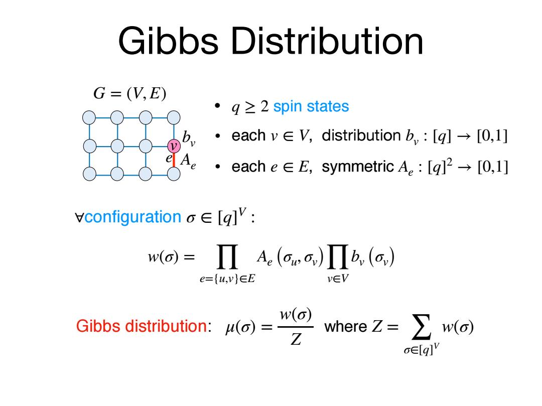
Gibbs Distribution G=V,E) ·q≥2 spin states ·each v∈V,distribution b,:[q]→[0,l] Ae·each e∈E,symmetric A:[q]2→[0,l] ∀configuration o∈[glV: w(o)=A(o,o,)Πb,(o,) e={u,v}∈E v∈V Gibbs distribution:u(o)= where Z= Z ∑w(o) aElg]v
Gibbs Distribution w(σ) = ∏ e={u,v}∈E Ae (σu, σv)∏ v∈V bv (σv) e v bv Ae G = (V, E) • spin states • each , distribution • each , symmetric q ≥ 2 v ∈ V bv : [q] → [0,1] e ∈ E Ae : [q] 2 → [0,1] ∀configuration σ ∈ [q] V : Gibbs distribution: μ(σ) = where w(σ) Z Z = ∑ σ∈[q] V w(σ)
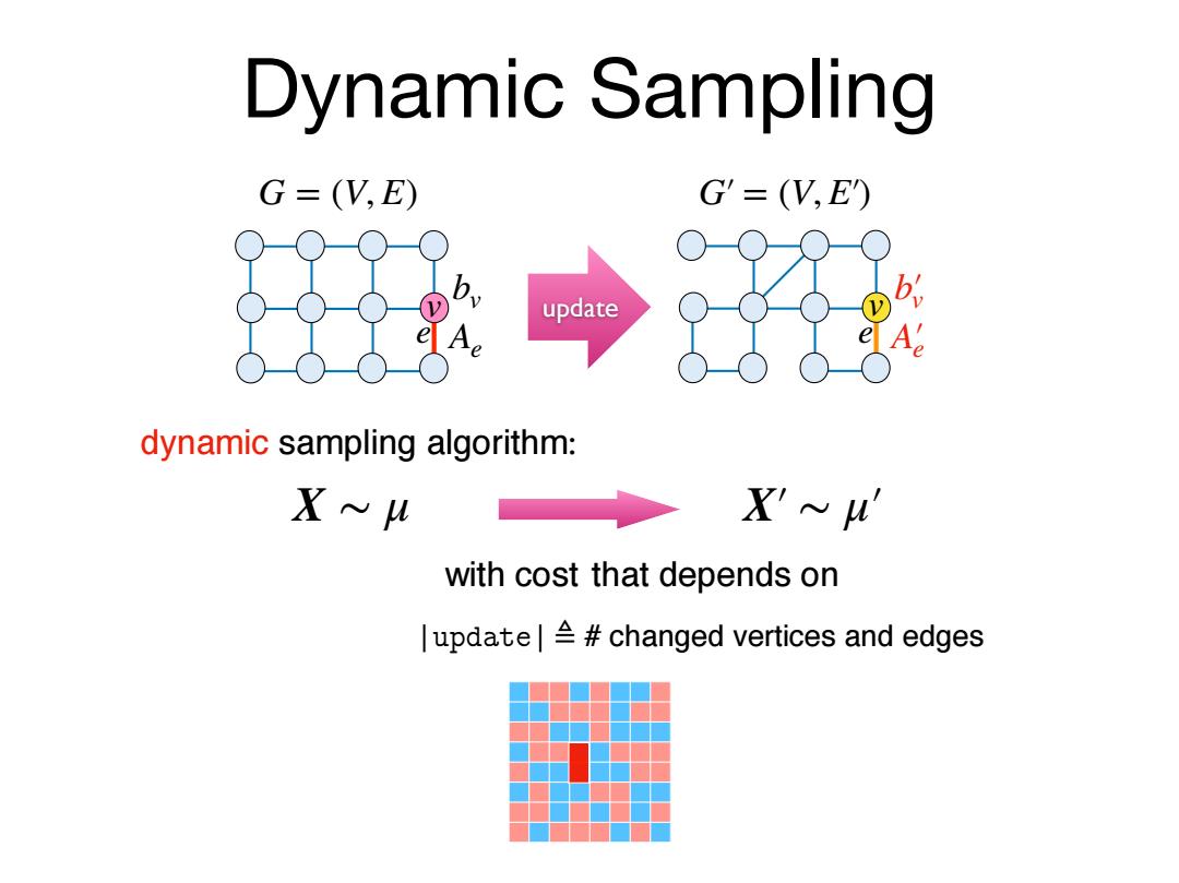
Dynamic Sampling G=(V,E) G'=(V,E) update A dynamic sampling algorithm: Xベu X'u with cost that depends on |update#changed vertices and edges
that depends on Dynamic Sampling e v bv Ae G = (V, E) e v b′ v A′ e G′ = (V, E′) update dynamic sampling algorithm: X ∼ μ X′ ∼ μ′ with cost |������| ≜ # changed vertices and edges
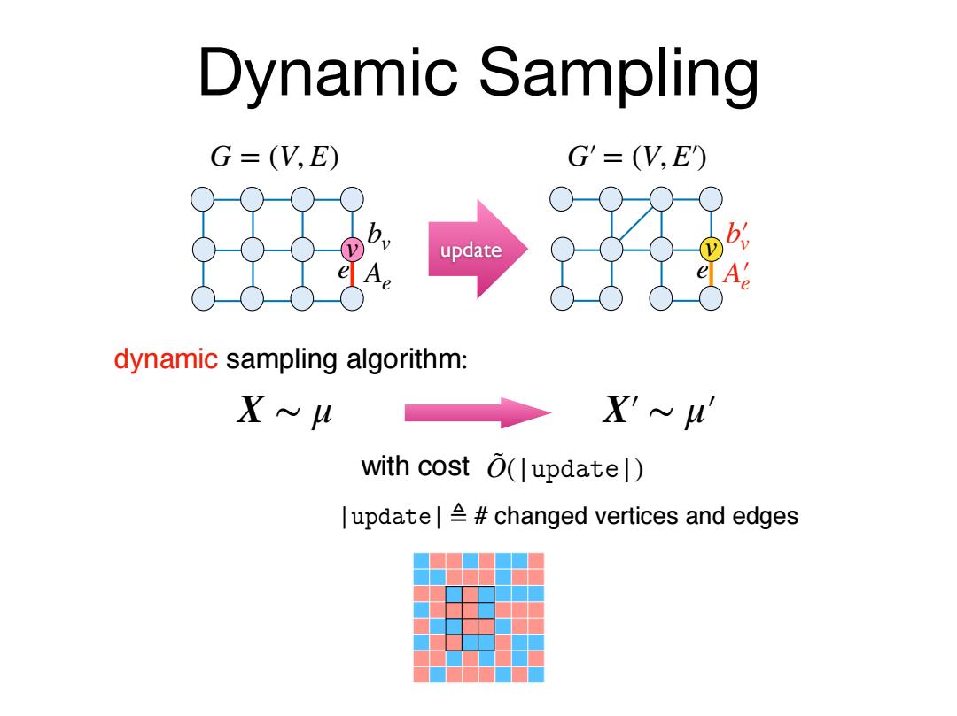
Dynamic Sampling G=(V,E) G'=(V,E) update A dynamic sampling algorithm: X~u X'ベu with cost O(|updatel) |update#changed vertices and edges
Dynamic Sampling e v bv Ae G = (V, E) e v b′ v A′ e G′ = (V, E′) update dynamic sampling algorithm: X ∼ μ X′ ∼ μ′ with cost |������| ≜ # changed vertices and edges O˜(|������|)
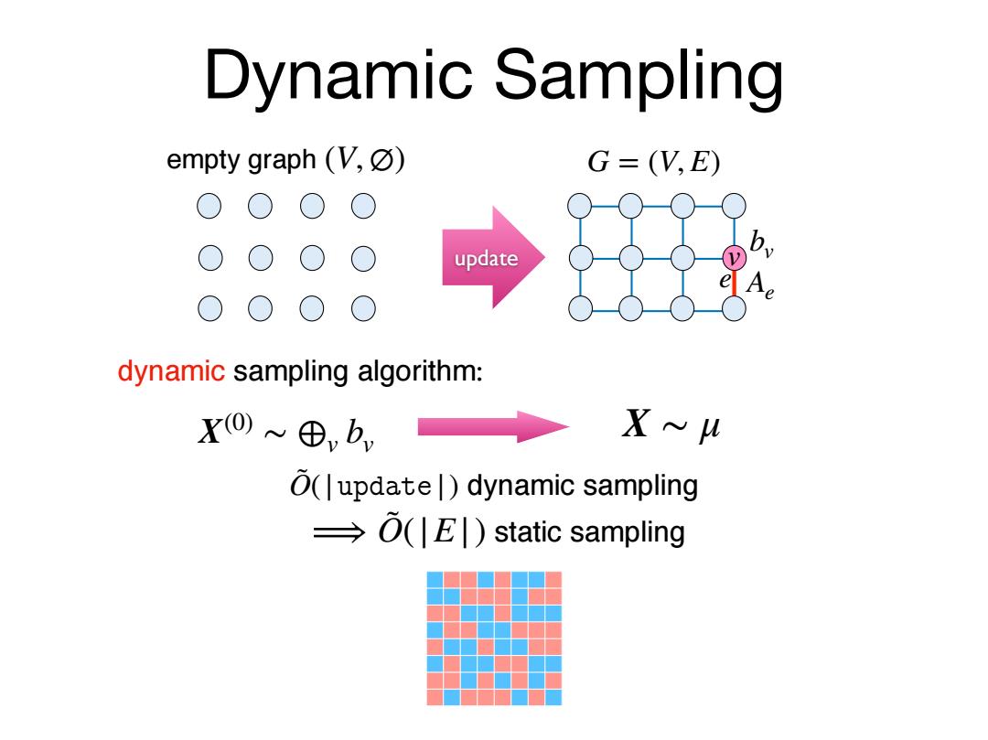
Dynamic Sampling empty graph(V,☑) G=V,E) update dynamic sampling algorithm: X0)~⊕,b, Xu O(|update|)dynamic sampling (E)static sampling
e v bv Ae G = (V, E) Dynamic Sampling update dynamic sampling algorithm: X ∼ μ dynamic sampling static sampling O˜(|������|) ⟹ O˜(|E|) empty graph (V, ∅) X(0) ∼ ⊕v bv
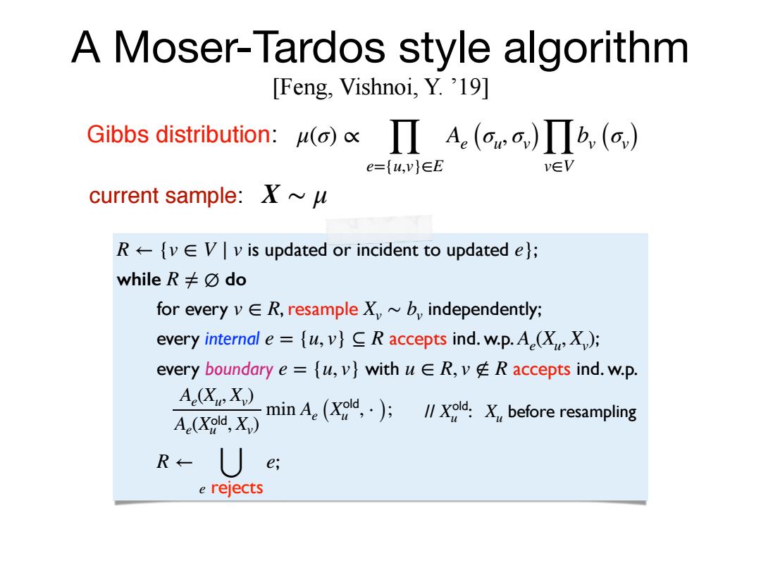
A Moser-Tardos style algorithm [Feng,Vishnoi,Y.'19] Gibbs distribution:u(o)cxΠAe(owo,)Πb,(a,) e={u,v}∈E v∈V current sample:X R←-{v∈V|v is updated or incident to updated e; while R≠☑do for every v ER,resample X~b,independently; every internal e={u,v}CR accepts ind.w.p.A(XX); every boundary e={u,v}with uR,vR accepts ind.w.p. Ae(XicX) Ae(Xed,X)) min Ae(Xod,·))方∥Xga:X,before resampling R←U e; e rejects
A Moser-Tardos style algorithm ; while do for every , resample independently; every internal accepts ind. w.p. ; every boundary with accepts ind. w.p. ; R ← {v ∈ V ∣ v is updated or incident to updated e} R ≠ ∅ v ∈ R Xv ∼ bv e = {u, v} ⊆ R Ae(Xu, Xv) e = {u, v} u ∈ R, v ∉ R R ← ⋃ e rejects e Ae(Xu, Xv) Ae(X��� u , Xv) min Ae (X��� u , ⋅ ); // X : before resampling ��� u Xu Gibbs distribution: μ(σ) ∝ ∏ e={u,v}∈E Ae (σu, σv)∏ v∈V bv (σv) current sample: X ∼ μ [Feng, Vishnoi, Y. ’19]

A Moser-Tardos style algorithm [Feng,Vishnoi,Y.'19] Gibbs distribution:u(o)cxΠAe(ooo,)Ib,(a) e={u,v}∈E v∈V current sample:Xu R←-{v∈V|v is updated or incident to updated e; while R≠odo for every vE R,resample X~b,independently; every internal e={u,v)CR accepts ind.w.p.A(X); every boundary e={u,v}with uR,vR accepts ind.w.p. A(,X) A(Xold,X) /Xold:X before resampling R← e; e rejects
A Moser-Tardos style algorithm ; while do for every , resample independently; every internal accepts ind. w.p. ; every boundary with accepts ind. w.p. ; R ← {v ∈ V ∣ v is updated or incident to updated e} R ≠ ∅ v ∈ R Xv ∼ bv e = {u, v} ⊆ R Ae(Xu, Xv) e = {u, v} u ∈ R, v ∉ R R ← ⋃ e rejects e // X : before resampling ��� ∝ u Xu Ae(Xu, Xv) Ae(X��� u , Xv) ; Gibbs distribution: μ(σ) ∝ ∏ e={u,v}∈E Ae (σu, σv)∏ v∈V bv (σv) current sample: X ∼ μ [Feng, Vishnoi, Y. ’19]

Rejection Sampling Gibbs distribution:()A()b ( e={u,v}∈E v∈V Rejection sampling: (XR=) for every v E R,sample X~b independently; every edge e={u,v}EE accepts independently w.p.A(X); R←Ue e rejects
Rejection Sampling for every , sample independently; every edge accepts independently w.p. ; v ∈ R Xv ∼ bv e = {u, v} ∈ E Ae(Xu, Xv) R ← ⋃ e rejects e Gibbs distribution: μ(σ) ∝ ∏ e={u,v}∈E Ae (σu, σv)∏ v∈V bv (σv) Rejection sampling: (X ∣ R = ∅) ∼ μ
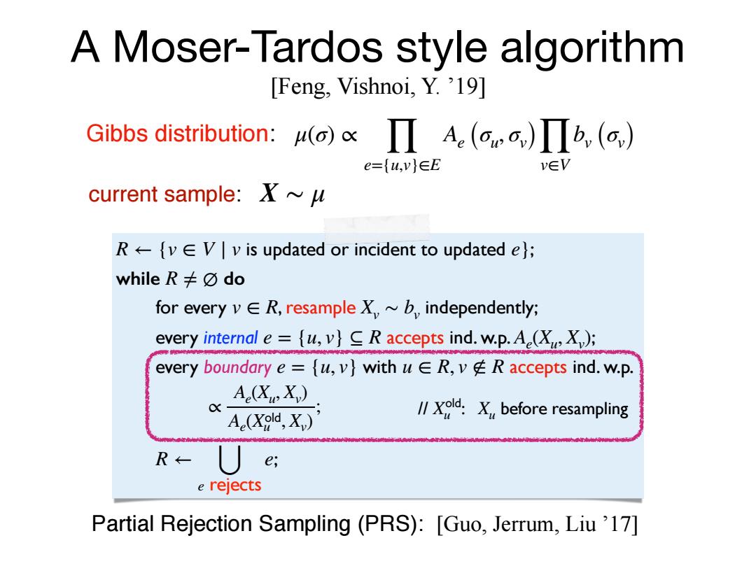
A Moser-Tardos style algorithm [Feng,Vishnoi,Y.'19] Gibbs distribution:u()A()b,( e={u,v}∈E v∈V current sample:Xu R←{v∈V|v is updated or incident to updated e; while R≠Odo for every v E R,resample X,~b,independently; every internal e=(u,v}CR accepts ind.w.p.A(X); every boundary e={u,v}with uER,vR accepts ind.w.p. Ae(XcX) Ae(Xold,X) /Xold:X before resampling R← e; e rejects Partial Rejection Sampling (PRS):[Guo,Jerrum,Liu'17]
A Moser-Tardos style algorithm ; while do for every , resample independently; every internal accepts ind. w.p. ; every boundary with accepts ind. w.p. ; R ← {v ∈ V ∣ v is updated or incident to updated e} R ≠ ∅ v ∈ R Xv ∼ bv e = {u, v} ⊆ R Ae(Xu, Xv) e = {u, v} u ∈ R, v ∉ R R ← ⋃ e rejects e // X : before resampling ��� u Xu Gibbs distribution: μ(σ) ∝ ∏ e={u,v}∈E Ae (σu, σv)∏ v∈V bv (σv) current sample: X ∼ μ [Feng, Vishnoi, Y. ’19] Partial Rejection Sampling (PRS): [Guo, Jerrum, Liu ’17] ∝ Ae(Xu, Xv) Ae(X��� u , Xv) ;

A heat-bath based algorithm [Feng,Guo,Y.'19] ibbs distribution:u(o)cΠAe(o,a,)Πb,(a,) e={u,v}∈E v∈V current sample:u RvVv is updated or incident to updated e); while R≠☑do pick a random u∈R; constant factor depends only on with probability do ur(XuI XN) XRONG) resampleIXND): heat-bath delete u from R; a.k.a.Glauber dynamics Gibbs sampling else add all neighbors of u to R; N(w≌neighborhood of u
A heat-bath based algorithm ; while do pick a random ; with probability do resample ; delete from ; else add all neighbors of to ; R ← {v ∈ V ∣ v is updated or incident to updated e} R ≠ ∅ u ∈ R ∝ 1 μu(Xu ∣ XN(u)) Xu ∼ μu( ⋅ ∣ XN(u) ) u R u R heat-bath a.k.a. Glauber dynamics Gibbs sampling constant factor depends only on XR∩N(u) [Feng, Guo, Y. ’19] Gibbs distribution: μ(σ) ∝ ∏ e={u,v}∈E Ae (σu, σv)∏ v∈V bv (σv) current sample: X ∼ μ N(u) ≜ neighborhood of u