
Deterministic radio propagation modeling and ray tracing 1) Introduction to deterministic propagation modelling 2) Geometrical Theory of Propagation I-The ray concept-Reflection and transmission 3) Geometrical Theory of Propagation II-Diffraction,multipath 4) Ray Tracing I 5) Ray Tracing II-Diffuse scattering modelling 6) Deterministic channel modelling I 7) Deterministic channel modelling II-Examples 8) Project -discussion
1 Deterministic radio propagation modeling and ray tracing 1) Introduction to deterministic propagation modelling 2) Geometrical Theory of Propagation I - The ray concept – Reflection and transmission 3) Geometrical Theory of Propagation II - Diffraction, multipath 4) Ray Tracing I 5) Ray Tracing II – Diffuse scattering modelling 6) Deterministic channel modelling I 7) Deterministic channel modelling II – Examples 8) Project - discussion

Using ray tracing(1/2) 。 Ray tracing(RT)is not only a prediction tool,is a realistic multipath propagation model.Therefore using ray tracing doesn't only mean getting coverage or prediction results.As far as the model is realistic,it also allows simulation, study,analysis of the urban multipath propagation phenomenon. RT(or ray launching)is also the most accurate prediction model now available. In terms of radio coverage prediction,a mean error of a fraction ofdB and a stdev of the error of 5-7 dB are achievable in practice. Although RT isn't an empirical model,some run parameters must be set before running RT.The following is a list of typical parameter values for outdoor prediction in european cities Control string:3@***@2dls which means: Nev-3 max.2 diffractions max.I scattering Material parameters:e,=5,s-0.01 [S/m](for all building walls) Coherent mode 2
2 • Ray tracing (RT) is not only a prediction tool, is a realistic multipath propagation model. Therefore using ray tracing doesn’t only mean getting coverage or prediction results. As far as the model is realistic, it also allows simulation, study, analysis of the urban multipath propagation phenomenon. • RT (or ray launching) is also the most accurate prediction model now available. In terms of radio coverage prediction, a mean error of a fraction of dB and a stdev of the error of 5-7 dB are achievable in practice. • Although RT isn’t an empirical model, some run parameters must be set before running RT. The following is a list of typical parameter values for outdoor prediction in european cities Using ray tracing (1/2) Control string: 3@***@2d1s which means: Nev=3 max. 2 diffractions max. 1 scattering Material parameters: er =5, s=0.01 [S/m] (for all building walls) Coherent mode
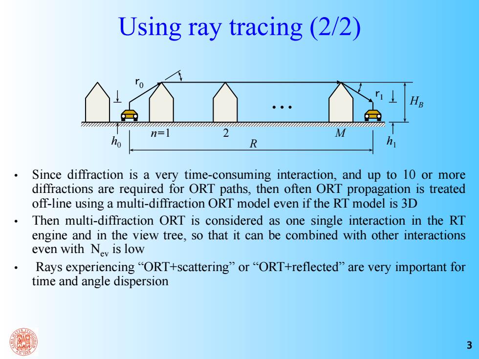
Using ray tracing (2/2) HB n=] 2 h R h Since diffraction is a very time-consuming interaction,and up to 10 or more diffractions are required for ORT paths,then often ORT propagation is treated off-line using a multi-diffraction ORT model even if the RT model is 3D Then multi-diffraction ORT is considered as one single interaction in the RT engine and in the view tree,so that it can be combined with other interactions even with Nev is low Rays experiencing"ORT+scattering"or"ORT+reflected"are very important for time and angle dispersion 3
3 • Since diffraction is a very time-consuming interaction, and up to 10 or more diffractions are required for ORT paths, then often ORT propagation is treated off-line using a multi-diffraction ORT model even if the RT model is 3D • Then multi-diffraction ORT is considered as one single interaction in the RT engine and in the view tree, so that it can be combined with other interactions even with Nev is low • Rays experiencing “ORT+scattering” or “ORT+reflected” are very important for time and angle dispersion Using ray tracing (2/2) r1 r0 h0 h R 1 n=1 2 M HB
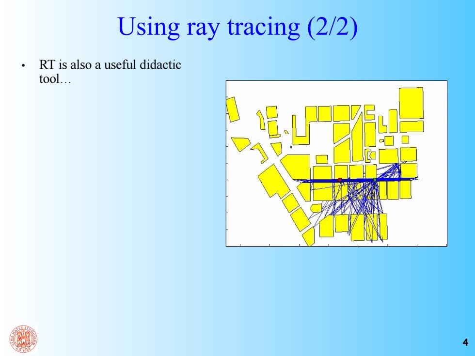
Using ray tracing(2/2) RT is also a useful didactic tool... 4
4 Using ray tracing (2/2) • RT is also a useful didactic tool…
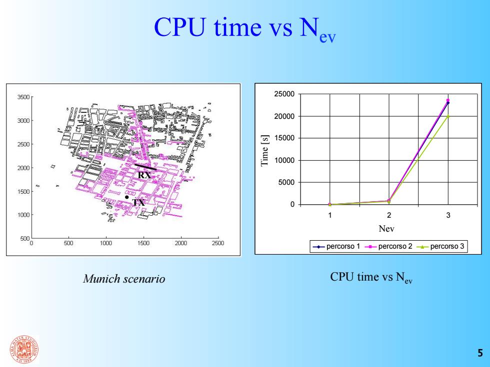
CPU time vs Nev 3500 25000 3000 20000 15000 250 10000 2000 5000 1501 0 100 Nev 500 500 1000 1500 2000 2500 -percorso 1--percorso 2--percorso 3 Munich scenario CPU time vs Nev 5
5 CPU time vs Nev Munich scenario CPU time vs Nev 0 5000 10000 15000 20000 25000 1 2 3 n eventi tempo (s) percorso 1 percorso 2 percorso 3 Nev Time [s] TX RX
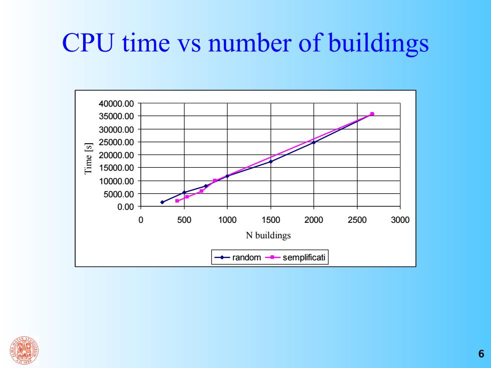
CPU time vs number of buildings 40000.00 35000.00 30000.00 25000.00 20000.00 15000.00 10000.00 5000.00 0.00 0 500 1000 1500 2000 2500 3000 N buildings -random--semplificati 6
6 CPU time vs number of buildings 0.00 5000.00 10000.00 15000.00 20000.00 25000.00 30000.00 35000.00 40000.00 0 500 1000 1500 2000 2500 3000 n' edifici tempo (sec) random semplificati N buildings Time [s]
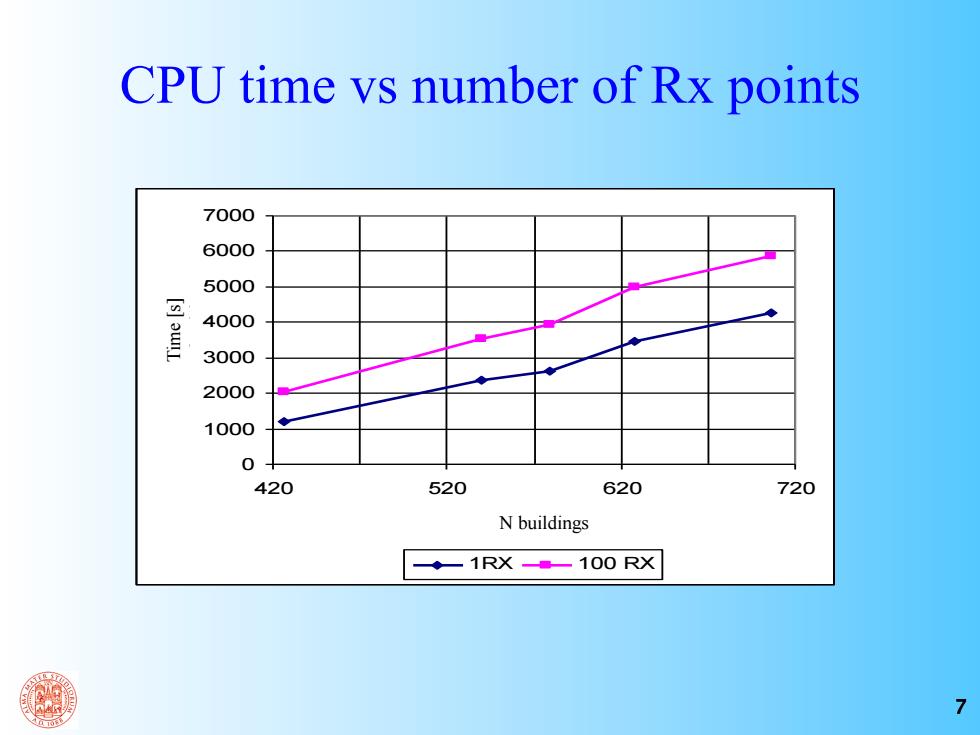
CPU time vs number of Rx points 7000 6000 5000 西 4000 3000 2000 1000 0 420 520 620 720 N buildings ◆1RX。100RX 7
7 CPU time vs number of Rx points 0 1000 2000 3000 4000 5000 6000 7000 420 520 620 720 n° edifici tempo (s) 1RX 100 RX Time [s] N buildings
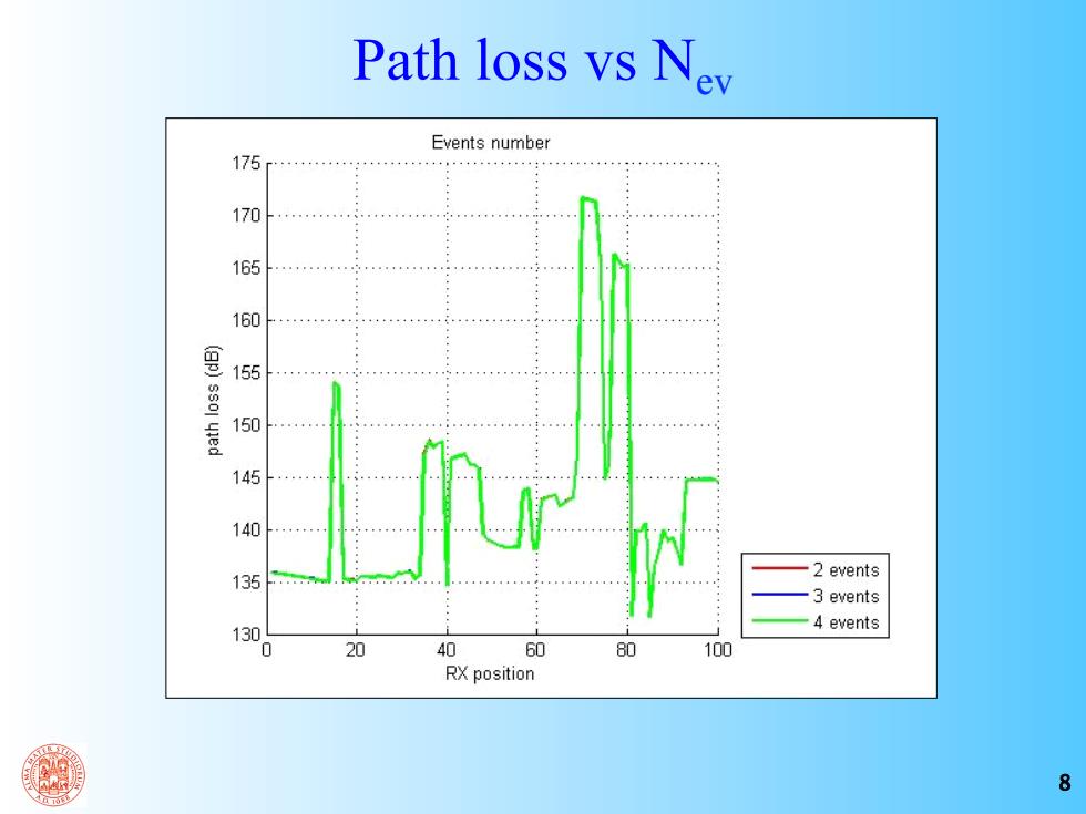
Path loss vs Nev Events number 175 170 … 165 160 (gp)ssol yied 155 150 : 145 140 135 2 events 3 events 130 4 events 20 40 60 80 100 RX position 8
8 Path loss vs Nev
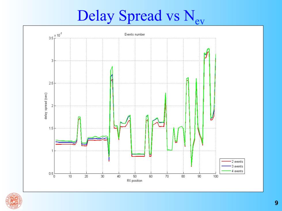
Delay Spread vs N 35102 Events number 2 1.5 2 events -3 events 4 events 050 50 100 RX position 9
9 Delay Spread vs Nev

Azimuth Spread vs Nev Events number 40 35 30 (aa6ap)peads yinwize 25 20 15 10 5 -2 events -3 events 4 events 0 20 40 60 80 100 RX position 10
10 Azimuth Spread vs Nev