
Fast quantum algorithms for Least Squares Regression and Statistic Leverage Scores Yang Liu Shengyu Zhang The Chinese University of Hong Kong
Yang Liu Shengyu Zhang The Chinese University of Hong Kong Fast quantum algorithms for Least Squares Regression and Statistic Leverage Scores
Part 1.Linear regression -Output a“quantum sketch”of solution. Part ll.Computing leverage scores and matrix coherence. Output the target numbers
• Part I. Linear regression – Output a “quantum sketch” of solution. • Part II. Computing leverage scores and matrix coherence. – Output the target numbers
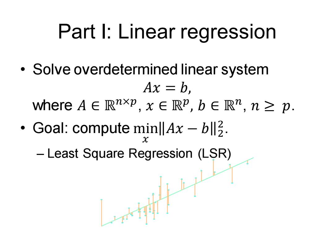
Part I:Linear regression Solve overdetermined linear system Ax =b, where A∈Rnxp,x∈RP,b∈Rn,n≥p. Goal:compute minllAx-bll. X Least Square Regression (LSR)
Part I: Linear regression • Solve overdetermined linear system 𝐴𝑥 = 𝑏, where 𝐴 ∈ ℝ𝑛×𝑝 , 𝑥 ∈ ℝ𝑝 , 𝑏 ∈ ℝ𝑛 , 𝑛 ≥ 𝑝. • Goal: compute min 𝑥 𝐴𝑥 − 𝑏 2 2 . – Least Square Regression (LSR)
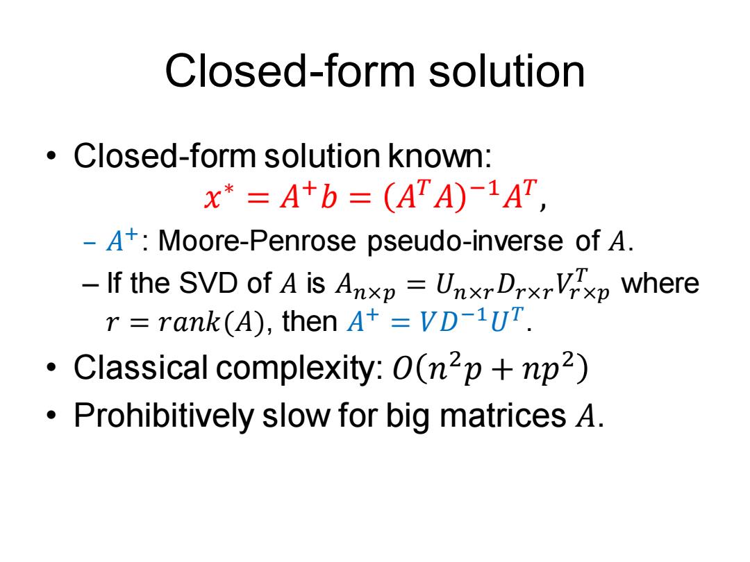
Closed-form solution Closed-form solution known: x*=A+b=(AA)1AT, -A+:Moore-Penrose pseudo-inverse of A. If the SVD of A is Anxp UnxrDrxrVTxp where r rank(A),then A+VD-1UT. Classical complexity:0(n2p +np2) Prohibitively slow for big matrices A
Closed-form solution • Closed-form solution known: 𝑥 ∗ = 𝐴 +𝑏 = 𝐴 𝑇𝐴 −1𝐴 𝑇 , – 𝐴 +: Moore-Penrose pseudo-inverse of 𝐴. – If the SVD of 𝐴 is 𝐴𝑛×𝑝 = 𝑈𝑛×𝑟𝐷𝑟×𝑟𝑉𝑟×𝑝 𝑇 where 𝑟 = 𝑟𝑎𝑛𝑘(𝐴), then 𝐴 + = 𝑉𝐷 −1𝑈 𝑇 . • Classical complexity: 𝑂 𝑛 2𝑝 + 𝑛𝑝 2 • Prohibitively slow for big matrices 𝐴
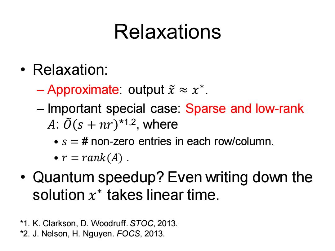
Relaxations 。Relaxation: -Approximate:outputx*. -Important special case:Sparse and low-rank A:0(s nr)*1,2,where .s =non-zero entries in each row/column. 。r=rank(A. Quantum speedup?Even writing down the solution x*takes linear time. *1.K.Clarkson,D.Woodruff.STOC,2013. *2.J.Nelson,H.Nguyen.FOCS,2013
Relaxations • Relaxation: – Approximate: output 𝑥 ≈ 𝑥 ∗ . – Important special case: Sparse and low-rank 𝐴: 𝑂෨ 𝑠 + 𝑛𝑟 * 1,2, where • 𝑠 = # non-zero entries in each row/column. • 𝑟 = 𝑟𝑎𝑛𝑘(𝐴) . • Quantum speedup? Even writing down the solution 𝑥 ∗ takes linear time. *1. K. Clarkson, D. Woodruff. STOC, 2013. *2. J. Nelson, H. Nguyen. FOCS, 2013
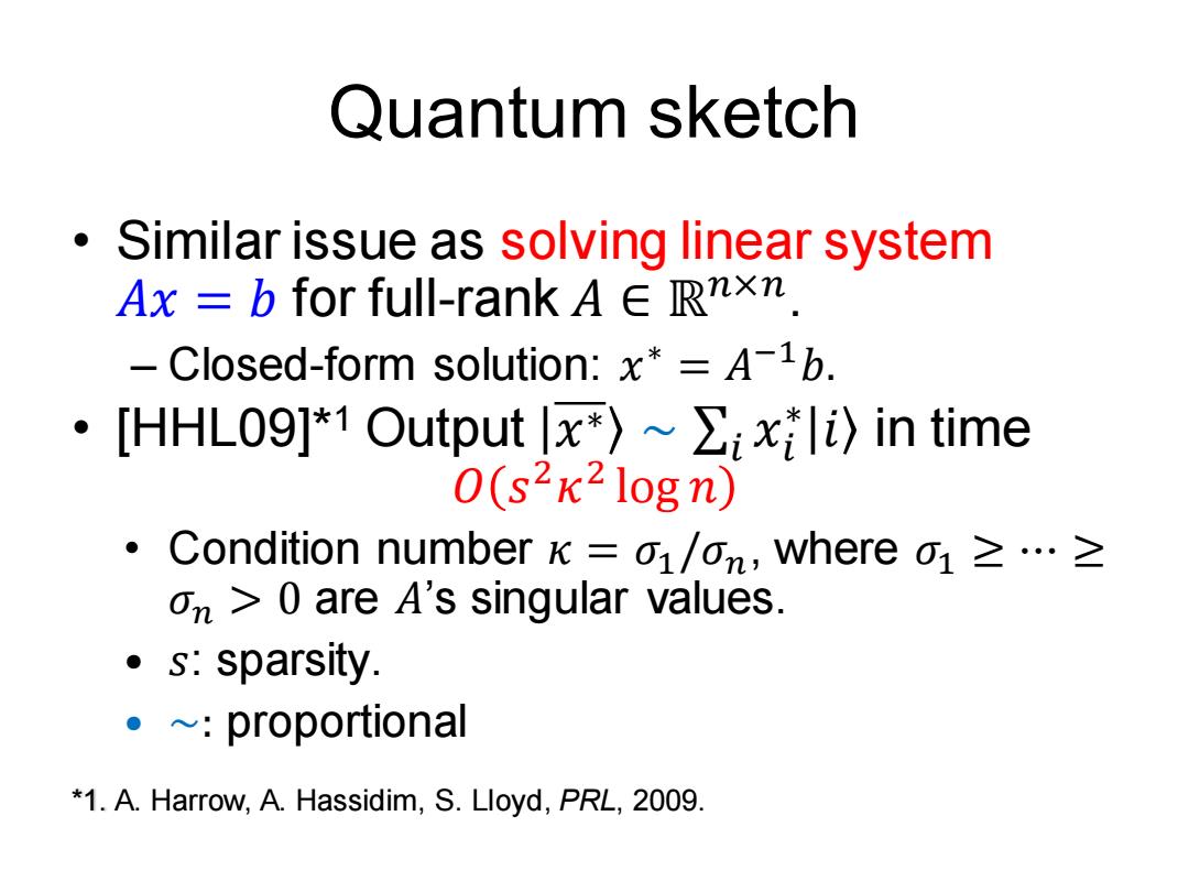
Quantum sketch Similar issue as solving linear system Ax b for full-rank A E Rxn. -Closed-form solution:x*=A-16. ·[HHL09]*1 Output x*)~∑ixli)in time 0(s2K2logn) ·Condition number x=o1/on,where o1≥·≥ on>0 are A's singular values. ·s:sparsity. 。~:proportional *1.A.Harrow,A.Hassidim,S.Lloyd,PRL,2009
Quantum sketch • Similar issue as solving linear system 𝐴𝑥 = 𝑏 for full-rank 𝐴 ∈ ℝ𝑛×𝑛 . – Closed-form solution: 𝑥 ∗ = 𝐴 −1𝑏. • [HHL09]*1 Output 𝑥 ∗ ∼ σ𝑖 𝑥𝑖 ∗ 𝑖 in time 𝑂 𝑠 2𝜅 2 log 𝑛 • Condition number 𝜅 = 𝜎1/𝜎𝑛, where 𝜎1 ≥ ⋯ ≥ 𝜎𝑛 > 0 are 𝐴’s singular values. • 𝑠: sparsity. • ∼: proportional *1. A. Harrow, A. Hassidim, S. Lloyd, PRL, 2009
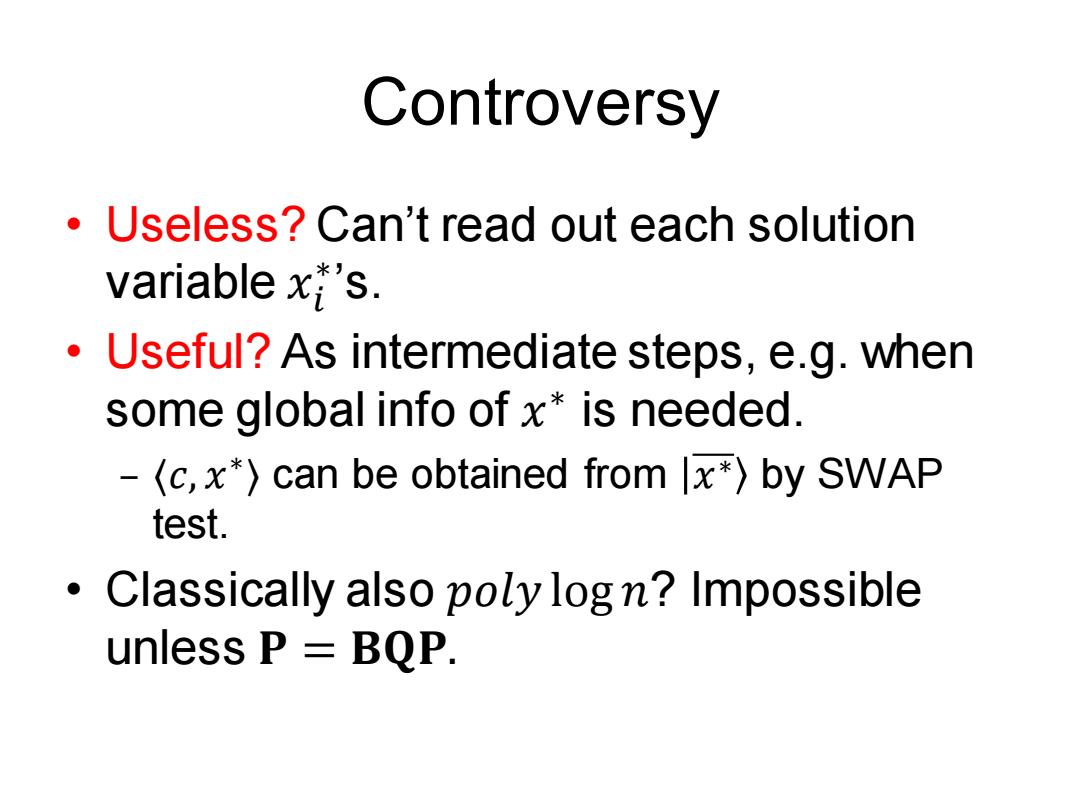
Controversy Useless?Can't read out each solution variable x's. Useful?As intermediate steps,e.g.when some global info of x*is needed. -(c,x*)can be obtained from x*)by SWAP test. ·Classically also poly log n?Impossible unless P BOP
Controversy • Useless? Can’t read out each solution variable 𝑥𝑖 ∗ ’s. • Useful? As intermediate steps, e.g. when some global info of 𝑥 ∗ is needed. – 〈𝑐, 𝑥 ∗ 〉 can be obtained from 𝑥 ∗ by SWAP test. • Classically also 𝑝𝑜𝑙𝑦 log 𝑛? Impossible unless 𝐏 = 𝐁𝐐𝐏
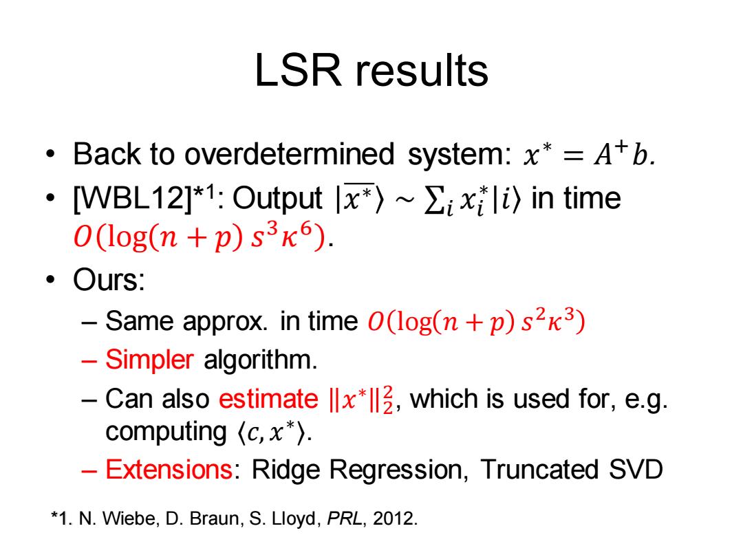
LSR results Back to overdetermined system:x*A+b. ·WBL12]*1:Output |x*)~Σix i)in time 0(1og(n+p)s3K6). 。OurS: Same approx.in time 0(log(n+p)s2K3) Simpler algorithm. Can also estimatex,which is used for,e.g. computing (c,x*). Extensions:Ridge Regression,Truncated SVD *1.N.Wiebe,D.Braun,S.Lloyd,PRL,2012
LSR results • Back to overdetermined system: 𝑥 ∗ = 𝐴 +𝑏. • [WBL12]*1 : Output 𝑥 ∗ ∼ σ𝑖 𝑥𝑖 ∗ 𝑖 in time 𝑂 log 𝑛 + 𝑝 𝑠 3𝜅 6 . • Ours: – Same approx. in time 𝑂 log 𝑛 + 𝑝 𝑠 2𝜅 3 – Simpler algorithm. – Can also estimate 𝑥 ∗ 2 2 , which is used for, e.g. computing 〈𝑐, 𝑥 ∗ 〉. – Extensions: Ridge Regression, Truncated SVD *1. N. Wiebe, D. Braun, S. Lloyd, PRL, 2012

Our algorithm for LSR 。Input:Hermition A∈Rnxn,b∈Rn.Assume A=2=1 vv:with1≥1之…之,≥ and the restλ;'sare0. Non-Hermition reduces to Hermition ·Output:Φ〉|)wWx≈x*,and≈lx*2: ·Note:Nrite b as b=iβ;lvi),then the desirable outputis
Our algorithm for LSR • Input: Hermition 𝐴 ∈ ℝ 𝑛×𝑛 , 𝑏 ∈ ℝ 𝑛 . Assume 𝐴 = σ𝑖=1 𝑛 𝜆𝑖 𝑣𝑖 𝑣𝑖 with 1 ≥ 𝜆1 ≥ ⋯ ≥ 𝜆𝑟 ≥ 1 𝜅 , and the rest 𝜆𝑖 ’s are 0. – Non-Hermition reduces to Hermition. • Output: 𝜙 ∼ |𝑥〉 w/ 𝑥 ≈ 𝑥 ∗ , and ℓ ≈ 𝑥 ∗ 2 2 . • Note: Write 𝑏 as 𝑏 = σ𝑖 𝛽𝑖 𝑣𝑖 , then the desirable output is 𝐴 +𝑏 = σ𝑖∈[𝑟] 𝛽𝑖 𝜆𝑖 𝑣𝑖

Algorithm Tool:Phase Estimation quantum algorithm. Output eigenvalue for a given eigenvector. ·Ib〉~∑nBil) PE Zein B:lv)lZi〉where元≈i c-xer1l0(2&I1)+VGI0) +∑i>rBlv)2I0〉》 ∥attach),rotate if元≥录 s~8r号m) /∥“select'"l1〉component PE,是IW.以wii*b
Algorithm • 𝑏 ∼ σ𝑖∈[𝑛] 𝛽𝑖 𝑣𝑖 𝑃𝐸 σ𝑖∈[𝑛] 𝛽𝑖 𝑣𝑖 |𝜆෩ 𝑖 〉 where 𝜆෩ 𝑖 ≈ 𝜆𝑖 𝐶−𝑅 σ𝑖≤𝑟 𝛽𝑖 𝑣𝑖 𝜆෩ 𝑖 1 2𝜅𝜆෩ 𝑖 1 + … 0 + σ𝑖>𝑟 𝛽𝑖 𝑣𝑖 𝜆෩ 𝑖 0 // attach 0 , rotate if 𝜆෩ 𝑖 ≥ 1 2𝜅 𝐴𝐴 ∼ σ𝑖≤𝑟 𝛽𝑖 𝜆𝑖 𝑣𝑖 𝜆෩ 𝑖 1 // “select” 1 component 𝑃𝐸 −1 ≈ σ𝑖≤𝑟 𝛽𝑖 𝜆𝑖 𝑣𝑖 , which is just 𝐴 +𝑏. Tool: Phase Estimation quantum algorithm. Output eigenvalue for a given eigenvector