NGG430Protaistics fonr Chapter 3:General Random Variables Instructor:Shengyu Zhang
Instructor: Shengyu Zhang
Content Continuous Random Variables and PDFs Cumulative Distribution Functions Normal Random Variables Joint PDFs of Multiple Random Variables Conditioning The Continuous Bayes'Rule
Content Continuous Random Variables and PDFs Cumulative Distribution Functions Normal Random Variables Joint PDFs of Multiple Random Variables Conditioning The Continuous Bayes’ Rule
Continuous Random Variables We've learned discrete random variables, which can be used for dice rolling,coin flipping,etc. Random variables with a continuous range of possible values are quite common. velocity of a vehicle traveling along the highway Continuous random variables are useful: finer-grained than discrete random variables able to exploit powerful tools from calculus
Continuous Random Variables We’ve learned discrete random variables, which can be used for dice rolling, coin flipping, etc. Random variables with a continuous range of possible values are quite common. velocity of a vehicle traveling along the highway Continuous random variables are useful: finer-grained than discrete random variables able to exploit powerful tools from calculus
Continuous r.v.and PDFs A random variable X is called continuous if there is a functionfx =0,called the probability density function of X,or PDF,s.t. P(X∈B)=fx(x)dx R for every subset B R. We assume the integral is well-defined Compared to discrete case:replace summation by integral
Continuous r.v. and PDFs A random variable 𝑋 is called continuous if there is a function 𝑓𝑋 ≥ 0, called the probability density function of 𝑋, or PDF, s.t. 𝑃 𝑋 ∈ 𝐵 = 𝑓𝑋 𝑥 𝑑𝑥 𝐵 for every subset 𝐵 ⊆ ℝ. We assume the integral is well-defined. Compared to discrete case: replace summation by integral
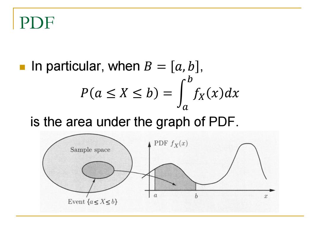
PDF In particular,when B [a,b], b pa≤X≤b)=x(x)dx is the area under the graph of PDF. PDF fx(x) Sample space b Event as Xsb}
PDF In particular, when 𝐵 = 𝑎, 𝑏 , 𝑃 𝑎 ≤ 𝑋 ≤ 𝑏 = 𝑓𝑋 𝑥 𝑑𝑥 𝑏 𝑎 is the area under the graph of PDF
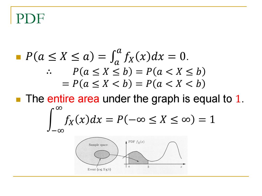
PDE ■P(a≤X≤a)=∫%fx(x)dx=0. P(a≤X≤b)=P(a<X≤b) =P(a≤X<b)=P(a<X<b) The entire area under the graph is equal to 1. 00 fx(x)dx=P(-oo≤X≤o)=1 -00 PDF fx(a) Sample space Event{a≤Xsb)
PDF 𝑃 𝑎 ≤ 𝑋 ≤ 𝑎 = 𝑓𝑋 𝑥 𝑑𝑥 𝑎 𝑎 = 0. ∴ 𝑃 𝑎 ≤ 𝑋 ≤ 𝑏 = 𝑃 𝑎 < 𝑋 ≤ 𝑏 = 𝑃 𝑎 ≤ 𝑋 < 𝑏 = 𝑃 𝑎 < 𝑋 < 𝑏 The entire area under the graph is equal to 1. 𝑓𝑋 𝑥 𝑑𝑥 ∞ −∞ = 𝑃 −∞ ≤ 𝑋 ≤ ∞ = 1
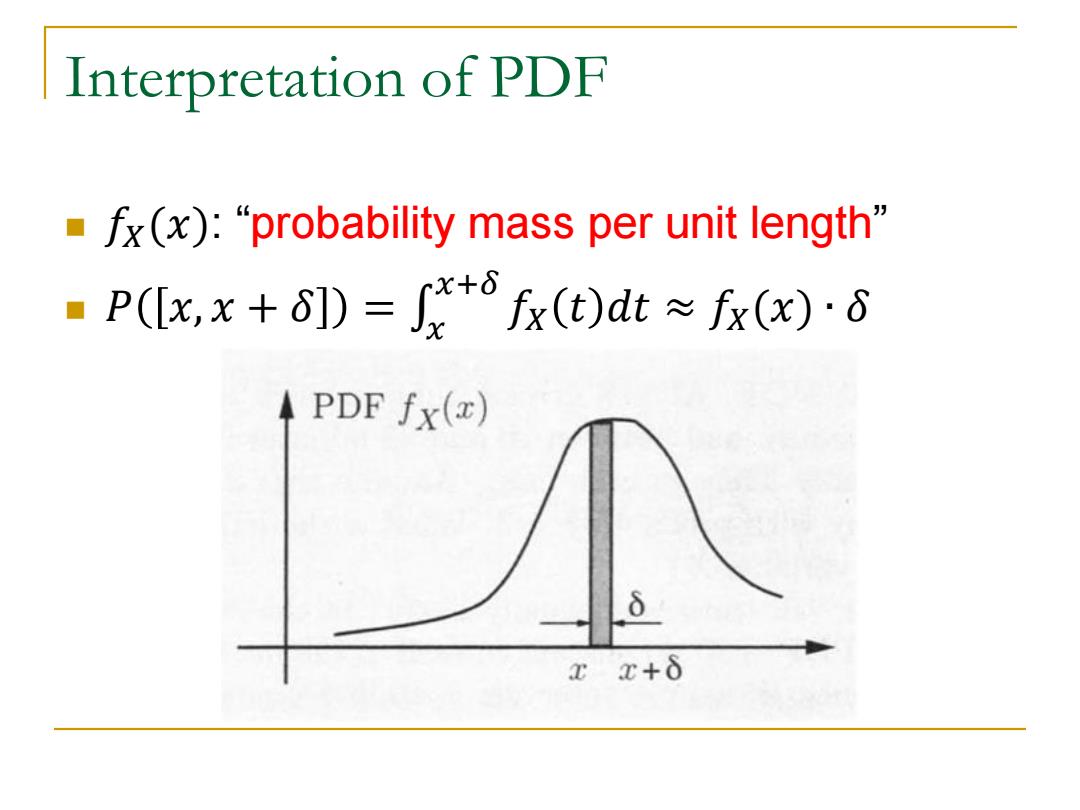
Interpretation of PDF ·fx(x):“probability mass per unit length” ■P(lx,x+D=+fx()at≈fr(x)G PDF fx(x) xE+δ
Interpretation of PDF 𝑓𝑋(𝑥): “probability mass per unit length” 𝑃 𝑥, 𝑥 + 𝛿 = 𝑓𝑋 𝑡 𝑑𝑡 𝑥+𝛿 𝑥 ≈ 𝑓𝑋(𝑥) ∙ 𝛿
Example 1:Uniform Consider a random variable X takes value in interval a,b]. Any subintervals of the same length have the same probability. It is called uniform random variable
Example 1: Uniform Consider a random variable 𝑋 takes value in interval 𝑎, 𝑏 . Any subintervals of the same length have the same probability. It is called uniform random variable
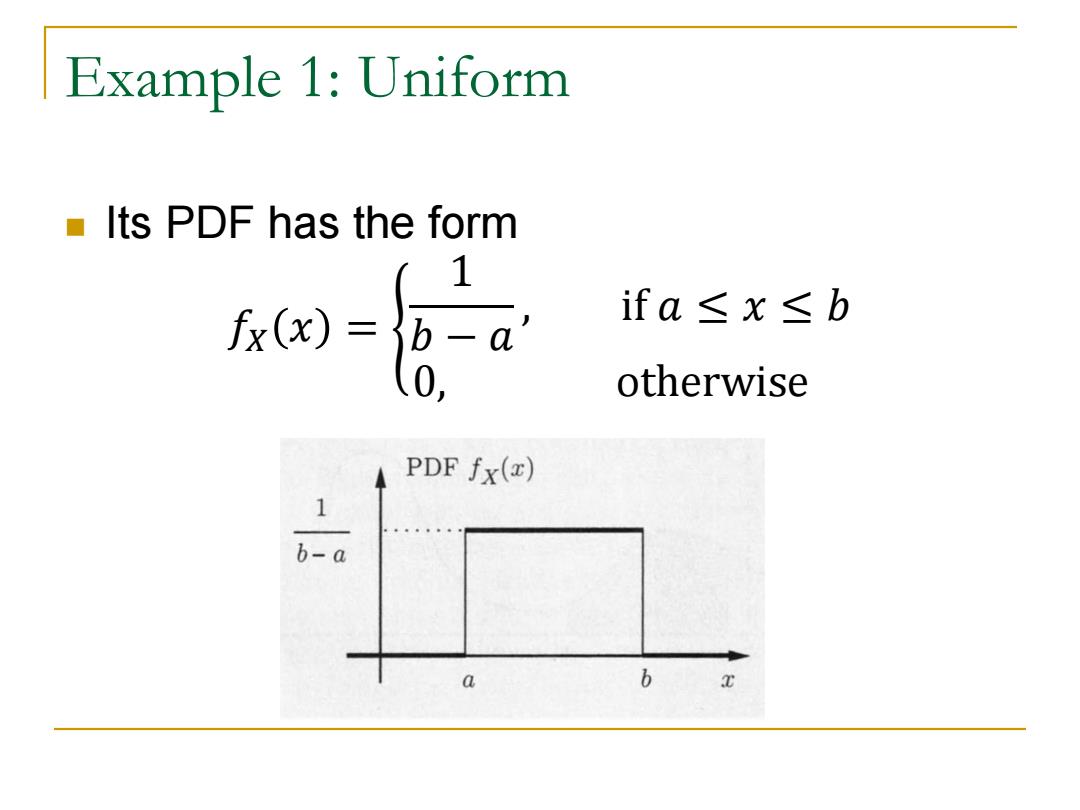
Example 1:Uniform Its PDF has the form ifa≤x≤b otherwise PDF fx(x) 1 b-a 0 b
Example 1: Uniform Its PDF has the form 𝑓𝑋 𝑥 = 1 𝑏 − 𝑎 , if 𝑎 ≤ 𝑥 ≤ 𝑏 0, otherwise
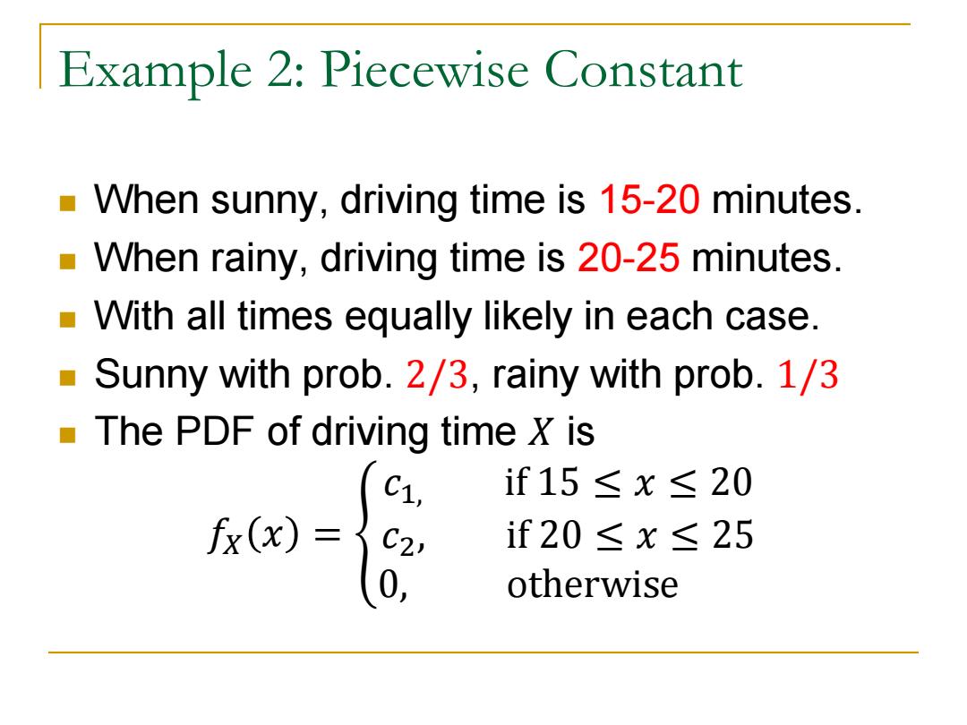
Example 2:Piecewise Constant When sunny,driving time is 15-20 minutes. When rainy,driving time is 20-25 minutes. With all times equally likely in each case. Sunny with prob.2/3,rainy with prob.1/3 The PDF of driving time X is C1, if15≤x≤20 fx(x)= C2, if20≤x≤25 0, otherwise
Example 2: Piecewise Constant When sunny, driving time is 15-20 minutes. When rainy, driving time is 20-25 minutes. With all times equally likely in each case. Sunny with prob. 2/3, rainy with prob. 1/3 The PDF of driving time 𝑋 is 𝑓𝑋 𝑥 = 𝑐1, if 15 ≤ 𝑥 ≤ 20 𝑐2, if 20 ≤ 𝑥 ≤ 25 0, otherwise