
Tutorial 3:Discrete Random Variables 1 Yihan Zhang and Baoxiang Wang Spring 2017
Tutorial 3: Discrete Random Variables 1 Yihan Zhang and Baoxiang Wang Spring 2017 1
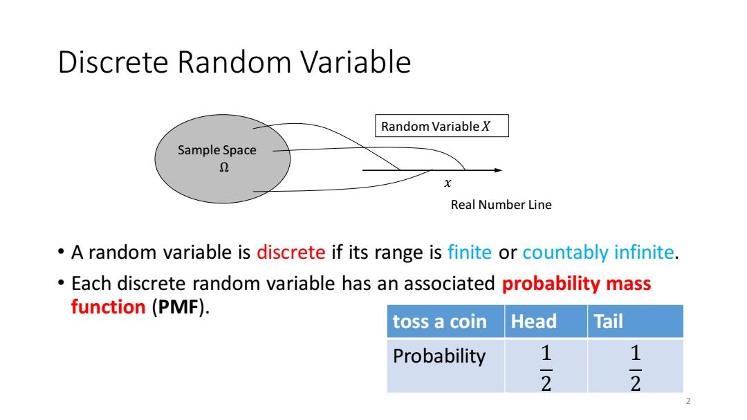
Discrete Random variable Random Variable X Sample Space 2 X Real Number Line A random variable is discrete if its range is finite or countably infinite. Each discrete random variable has an associated probability mass function(PMF). toss a coin Head Tail Probability 1 1 2 2 2
Discrete Random Variable • A random variable is discrete if its range is finite or countably infinite. • Each discrete random variable has an associated probability mass function (PMF). Sample Space Ω Random Variable 𝑋 𝑥 Real Number Line toss a coin Head Tail Probability 1 2 1 2 2
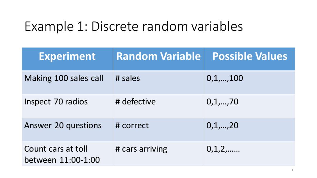
Example 1:Discrete random variables Experiment Random Variable Possible Values Making 100 sales call sales 0,1,…,100 Inspect 70 radios defective 0,1,,70 Answer 20 questions correct 0,1,,20 Count cars at toll cars arriving 0,1,2, between 11:00-1:00
Example 1: Discrete random variables Experiment Random Variable Possible Values Making 100 sales call # sales 0,1,…,100 Inspect 70 radios # defective 0,1,…,70 Answer 20 questions # correct 0,1,…,20 Count cars at toll between 11:00-1:00 # cars arriving 0,1,2,…… 3
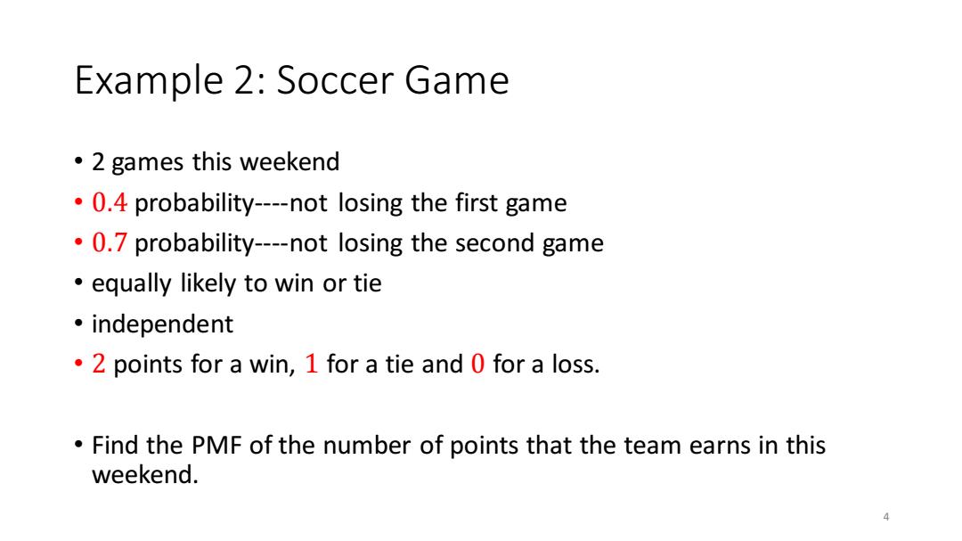
Example 2:Soccer Game ·2 games this weekend 0.4 probability----not losing the first game 0.7 probability----not losing the second game equally likely to win or tie 。independent 2 points for a win,1 for a tie and 0 for a loss. Find the PMF of the number of points that the team earns in this weekend
Example 2: Soccer Game • 2 games this weekend • 0.4 probability----not losing the first game • 0.7 probability----not losing the second game • equally likely to win or tie • independent • 2 points for a win, 1 for a tie and 0 for a loss. • Find the PMF of the number of points that the team earns in this weekend. 4
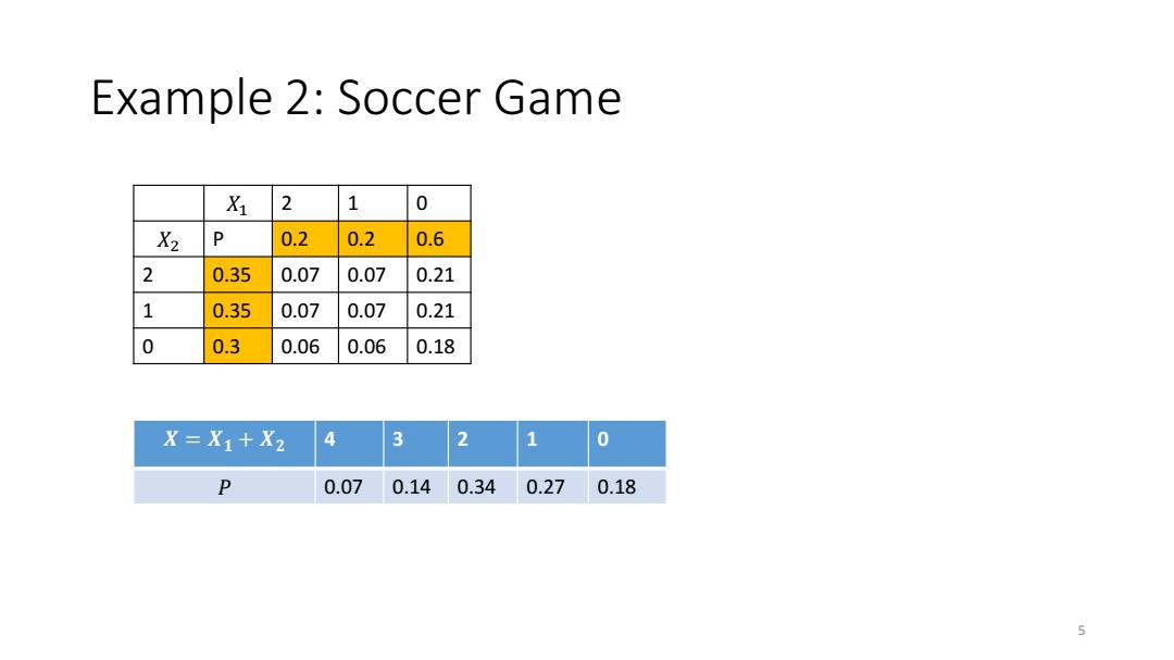
Example 2:Soccer Game X1 2 1 0 X2 P 0.2 0.2 0.6 2 0.35 0.07 0.07 0.21 1 0.35 0.07 0.07 0.21 0 0.3 0.06 0.06 0.18 X=X1+X2 4 3 2 1 0 P 0.07 0.140.34 0.27 0.18 5
Example 2: Soccer Game 𝑋1 2 1 0 𝑋2 P 0.2 0.2 0.6 2 0.35 0.07 0.07 0.21 1 0.35 0.07 0.07 0.21 0 0.3 0.06 0.06 0.18 𝑿 = 𝑿𝟏 + 𝑿𝟐 4 3 2 1 0 𝑃 0.07 0.14 0.34 0.27 0.18 5
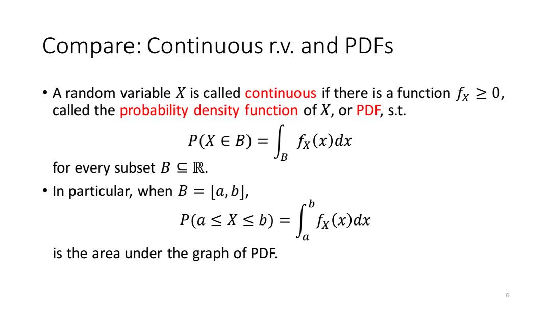
Compare:Continuous r.v.and PDFs A random variable X is called continuous if there is a functionfx>0, called the probability density function of X,or PDF,s.t. P(X∈B)=R()d for every subset B R. In particular,when B [a,b], P(a≤X≤b)=fx(x)dx is the area under the graph of PDF
Compare: Continuous r.v. and PDFs • A random variable 𝑋 is called continuous if there is a function 𝑓𝑋 ≥ 0, called the probability density function of 𝑋, or PDF, s.t. 𝑃(𝑋 ∈ 𝐵) = න 𝐵 𝑓𝑋 𝑥 𝑑𝑥 for every subset 𝐵 ⊆ ℝ. • In particular, when 𝐵 = [𝑎, 𝑏], 𝑃(𝑎 ≤ 𝑋 ≤ 𝑏) = න 𝑎 𝑏 𝑓𝑋 𝑥 𝑑𝑥 is the area under the graph of PDF. 6
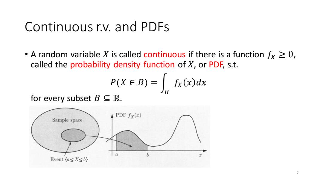
Continuous r.v.and PDFs A random variable X is called continuous if there is a functionfx>0, called the probability density function of X,or PDF,s.t. P(X∈B)=x(x)d for every subset B∈R. PDF fx(z) Sample space Event (as Xsb} 7
Continuous r.v. and PDFs • A random variable 𝑋 is called continuous if there is a function 𝑓𝑋 ≥ 0, called the probability density function of 𝑋, or PDF, s.t. 𝑃(𝑋 ∈ 𝐵) = න 𝐵 𝑓𝑋 𝑥 𝑑𝑥 for every subset 𝐵 ⊆ ℝ. 7

Typical Discrete Random Variables We review typical variables,and understand them using examples Binomial Random Variable Poisson Random Variable Poisson Limit Theorem 8
Typical Discrete Random Variables • We review typical variables, and understand them using examples • Binomial Random Variable • Poisson Random Variable • Poisson Limit Theorem 8
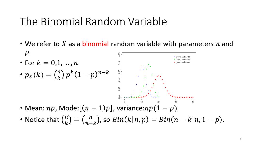
The Binomial Random variable We refer to X as a binomial random variable with parameters n and p. 。p-0.5andn-20 p=0.7ndn=20 。Fork=0,1,.,n ◆p-0.5andn-40 ·px(k)=(()pk(1-p)n-k Mean:np,Mode:[(n 1)p],variance:np(1-p) Notice that ()=()so Bin(kln,p)=Bin(n-kln,1-p). 9
The Binomial Random Variable • We refer to 𝑋 as a binomial random variable with parameters 𝑛 and 𝑝. • For 𝑘 = 0,1, … , 𝑛 • 𝑝𝑋(𝑘) = 𝑛 𝑘 𝑝 𝑘 1 − 𝑝 𝑛−𝑘 • Mean: 𝑛𝑝, Mode: 𝑛 + 1 𝑝 , variance:𝑛𝑝(1 − 𝑝) • Notice that 𝑛 𝑘 = 𝑛 𝑛−𝑘 , so 𝐵𝑖𝑛 𝑘 𝑛, 𝑝 = 𝐵𝑖𝑛 𝑛 − 𝑘 𝑛, 1 − 𝑝 . 9
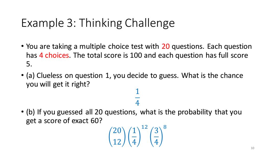
Example 3:Thinking Challenge You are taking a multiple choice test with 20 questions.Each question has 4 choices.The total score is 100 and each question has full score 5. .(a)Clueless on question 1,you decide to guess.What is the chance you will get it right? 1 4 .(b)If you guessed all 20 questions,what is the probability that you get a score of exact 60? 10
Example 3: Thinking Challenge • You are taking a multiple choice test with 20 questions. Each question has 4 choices. The total score is 100 and each question has full score 5. • (a) Clueless on question 1, you decide to guess. What is the chance you will get it right? 1 4 • (b) If you guessed all 20 questions, what is the probability that you get a score of exact 60? 20 12 1 4 12 3 4 8 10