clMSc5706TopicsinTheoreticalcomputerScience Week 2:Linear Programming Instructor:Shengyu Zhang 1
Instructor: Shengyu Zhang 1
LP Motivating examples Introduction to algorithms Simplex algorithm On a particular example General algorithm Duality An application to game theory 2
LP ◼ Motivating examples ◼ Introduction to algorithms ◼ Simplex algorithm ❑ On a particular example ❑ General algorithm ◼ Duality ◼ An application to game theory 2
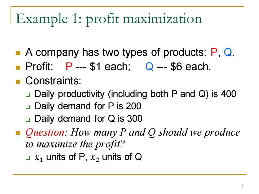
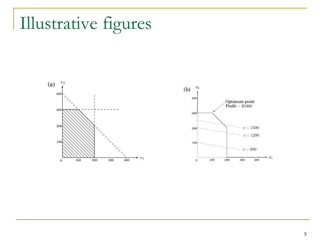
Example 1:profit maximization A company has two types of products:P,Q. ■Profit:P--$1each; Q---$6 each ■Constraints: Daily productivity (including both P and Q)is 400 Daily demand for P is 200 Daily demand for Q is 300 Question:How many P and O should we produce to maximize the profit? x1 units of P,xz units of Q 3
Example 1: profit maximization ◼ A company has two types of products: P, Q. ◼ Profit: P --- $1 each; Q --- $6 each. ◼ Constraints: ❑ Daily productivity (including both P and Q) is 400 ❑ Daily demand for P is 200 ❑ Daily demand for Q is 300 ◼ Question: How many P and Q should we produce to maximize the profit? ❑ 𝑥1 units of P, 𝑥2 units of Q 3
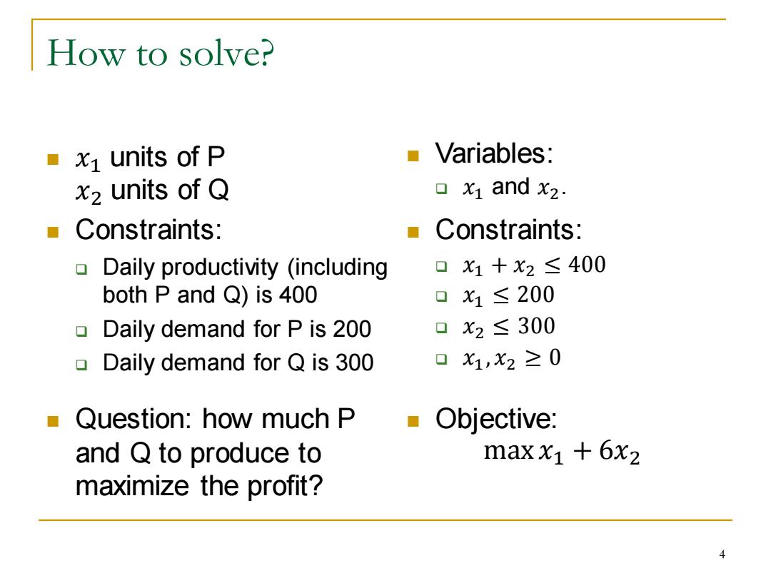
How to solve? ■x1 units of P Variables: x2 units of Q 口x1andx2. Constraints: Constraints: Daily productivity (including 口x1+x2≤400 both P and Q)is 400 x1≤200 Daily demand for P is 200 口 x2≤300 Daily demand for Q is 300 x1,X2≥0 Question:how much P Objective: and Q to produce to max x1+6x2 maximize the profit? 4
How to solve? ◼ 𝑥1 units of P 𝑥2 units of Q ◼ Constraints: ❑ Daily productivity (including both P and Q) is 400 ❑ Daily demand for P is 200 ❑ Daily demand for Q is 300 ◼ Question: how much P and Q to produce to maximize the profit? ◼ Variables: ❑ 𝑥1 and 𝑥2. ◼ Constraints: ❑ 𝑥1 + 𝑥2 ≤ 400 ❑ 𝑥1 ≤ 200 ❑ 𝑥2 ≤ 300 ❑ 𝑥1, 𝑥2 ≥ 0 ◼ Objective: max 𝑥1 + 6𝑥2 4
Illustrative figures (a) 2 (b) T2 400 400 Optimum point Profit=$1900 300 300 200 200 -、-、-c=1500 ----c=1200 5-.c=600 E1 100 200 300 400 100 200 300 400 1 5
Illustrative figures 5
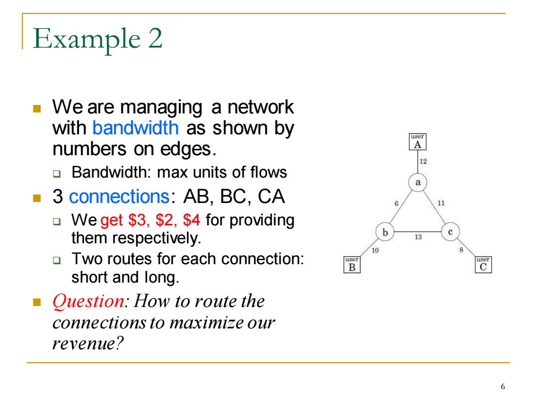
Example 2 We are managing a network with bandwidth as shown by numbers on edges. 12 Bandwidth:max units of flows a 3 connections:AB,BC,CA 6 11 口 We get $3,$2,$4 for providing them respectively. b 13 10 Two routes for each connection: B 冠 short and long. Question:How to route the connections to maximize our revenue? 6
Example 2 ◼ We are managing a network with bandwidth as shown by numbers on edges. ❑ Bandwidth: max units of flows ◼ 3 connections: AB, BC, CA ❑ We get $3, $2, $4 for providing them respectively. ❑ Two routes for each connection: short and long. ◼ Question: How to route the connections to maximize our revenue? 6
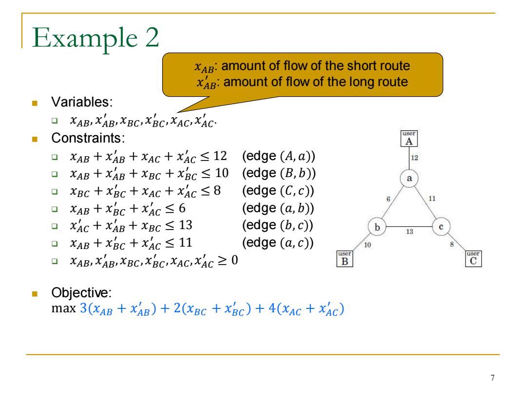
Example 2 xAB:amount of flow of the short route xA:amount of flow of the long route Variables: 0 XAB,XAB XBC,XBC,XAC,XAC- Constraints: A 口XAB+XAB+xAC+XAC≤12 (edge (A,a)) 12 口XAB+XAB+XBC+xBC≤10 (edge(B,b)) 口 XBC+XBC+XAC+XAC≤8 (edge (C,c)) 6 11 0 XAB+XBC+xAC≤6 (edge (a,b)) 0 XAC+xAB+XBC≤13 (edge (b,c)) b 13 xAB+xBc+x4c≤11 (edge (a,c)) 10 XAB,XAB,XBC,XBC,XAC,XAC>0 B 同 Objective: max 3(xAB +xAB)+2(xBC +xBc)+4(xAC +xAc) 7
Example 2 ◼ Variables: ❑ 𝑥𝐴𝐵, 𝑥𝐴𝐵 ′ ,𝑥𝐵𝐶,𝑥𝐵𝐶 ′ ,𝑥𝐴𝐶,𝑥𝐴𝐶 ′ . ◼ Constraints: ❑ 𝑥𝐴𝐵 + 𝑥𝐴𝐵 ′ + 𝑥𝐴𝐶 + 𝑥𝐴𝐶 ′ ≤ 12 (edge (𝐴, 𝑎)) ❑ 𝑥𝐴𝐵 + 𝑥𝐴𝐵 ′ + 𝑥𝐵𝐶 + 𝑥𝐵𝐶 ′ ≤ 10 (edge (𝐵, 𝑏)) ❑ 𝑥𝐵𝐶 + 𝑥𝐵𝐶 ′ + 𝑥𝐴𝐶 + 𝑥𝐴𝐶 ′ ≤ 8 (edge (𝐶, 𝑐)) ❑ 𝑥𝐴𝐵 + 𝑥𝐵𝐶 ′ + 𝑥𝐴𝐶 ′ ≤ 6 (edge (𝑎, 𝑏)) ❑ 𝑥𝐴𝐶 ′ + 𝑥𝐴𝐵 ′ + 𝑥𝐵𝐶 ≤ 13 (edge (𝑏, 𝑐)) ❑ 𝑥𝐴𝐵 + 𝑥𝐵𝐶 ′ + 𝑥𝐴𝐶 ′ ≤ 11 (edge (𝑎, 𝑐)) ❑ 𝑥𝐴𝐵, 𝑥𝐴𝐵 ′ ,𝑥𝐵𝐶,𝑥𝐵𝐶 ′ ,𝑥𝐴𝐶,𝑥𝐴𝐶 ′ ≥ 0 ◼ Objective: max 3(𝑥𝐴𝐵 + 𝑥𝐴𝐵 ′ ) + 2(𝑥𝐵𝐶 + 𝑥𝐵𝐶 ′ ) + 4(𝑥𝐴𝐶 + 𝑥𝐴𝐶 ′ ) 𝑥𝐴𝐵: amount of flow of the short route 𝑥𝐴𝐵 ′ : amount of flow of the long route 7
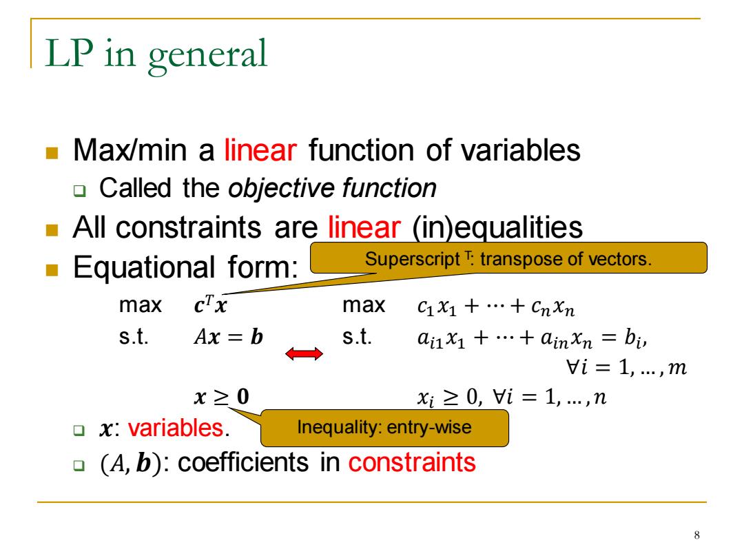
LP in general Max/min a linear function of variables Called the objective function All constraints are linear (in)equalities Equational form: Superscript transpose of vectors. max CTx max C1x1+…+Cnxn s.t. Ax=b s.t. ai1x1+…+ainxn=b Vi=1,…,m x≥0 x1≥0,i=1,.,n x:variables. Inequality:entry-wise (A,b):coefficients in constraints 8
LP in general ◼ Max/min a linear function of variables ❑ Called the objective function ◼ All constraints are linear (in)equalities ◼ Equational form: max 𝒄 𝑇𝒙 max 𝑐1𝑥1 + ⋯ + 𝑐𝑛𝑥𝑛 s.t. 𝐴𝒙 = 𝒃 s.t. 𝑎𝑖1𝑥1 + ⋯ + 𝑎𝑖𝑛𝑥𝑛 = 𝑏𝑖 , ∀𝑖 = 1, … , 𝑚 𝒙 ≥ 𝟎 𝑥𝑖 ≥ 0, ∀𝑖 = 1, … ,𝑛 ❑ 𝒙: variables. ❑ (𝐴, 𝒃): coefficients in constraints Superscript T: transpose of vectors. Inequality: entry-wise 8
Transformations between forms Min vs.max: ▣mincx台max-cfx Inequality directions: ▣aix≥b:台-ax≤-b1 Equalities to inequalities:(a;:row i in matrix A) oaix=b:台afx≥b,and ax≤b
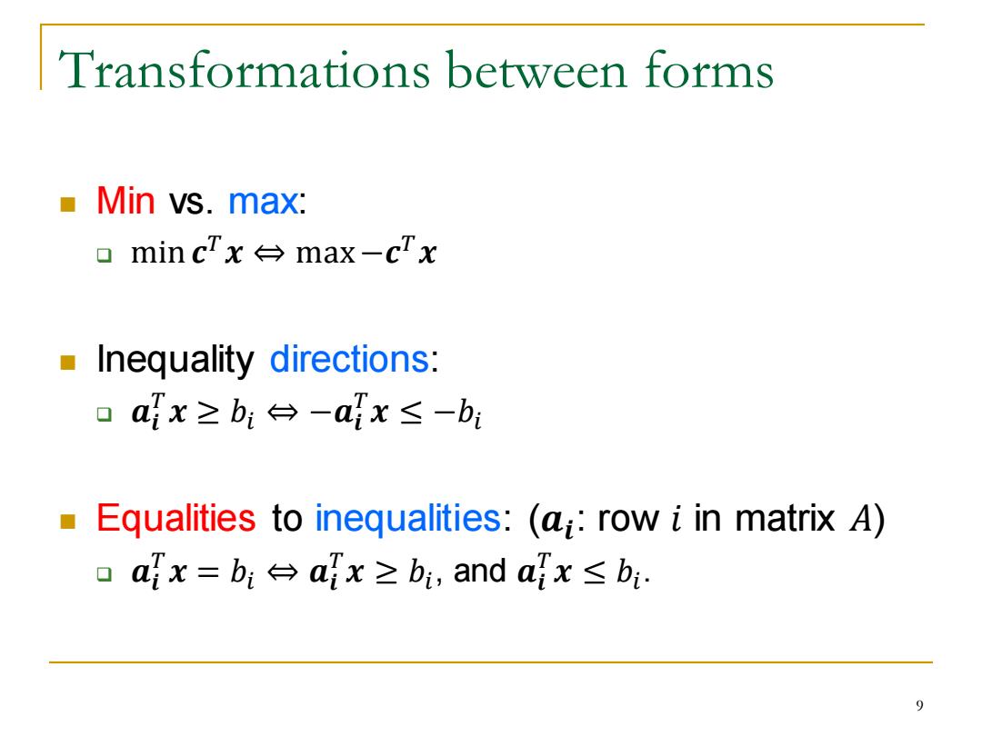
Transformations between forms ◼ Min vs. max: ❑ min 𝒄 𝑇𝒙 ⇔ max−𝒄 𝑇𝒙 ◼ Inequality directions: ❑ 𝒂𝒊 𝑇𝒙 ≥ 𝑏𝑖 ⇔ −𝒂𝒊 𝑇𝒙 ≤ −𝑏𝑖 ◼ Equalities to inequalities: (𝒂𝒊 : row 𝑖 in matrix 𝐴) ❑ 𝒂𝒊 𝑇𝒙 = 𝑏𝑖 ⇔ 𝒂𝒊 𝑇𝒙 ≥ 𝑏𝑖 , and 𝒂𝒊 𝑇𝒙 ≤ 𝑏𝑖 . 9

Transformations between forms Inequalities to equalities: ax≥b:台a{x=b:+Si,S:≥0 The newly introduced variable s;is called slack variable a“Unrestricted”to“nonnegative constraint'": ▣x;unrestricted台xi=s-t,s≥0,t≥0 10
Transformations between forms ◼ Inequalities to equalities: ❑ 𝒂𝒊 𝑇𝒙 ≥ 𝑏𝑖 ⇔ 𝒂𝒊 𝑇𝒙 = 𝑏𝑖 + 𝑠𝑖 , 𝑠𝑖 ≥ 0 ◼ The newly introduced variable 𝑠𝑖 is called slack variable ◼ “Unrestricted” to “nonnegative constraint”: ❑ 𝑥𝑖 unrestricted ⇔ 𝑥𝑖 = 𝑠– 𝑡, 𝑠 ≥ 0,𝑡 ≥ 0 10