
Tutorial 11:Limit Theorems Baoxiang Wang Yihan Zhang bxwang,yhzhang@cse.cuhk.edu.hk April 10,2017
Tutorial 11: Limit Theorems Baoxiang Wang & Yihan Zhang bxwang, yhzhang@cse.cuhk.edu.hk April 10, 2017 1

Outline The Central Limit Theorem(CLT) Normal Approximation Based on CLT De Moivre-Laplace Approximation to the Binomial Problems and solutions
Outline • The Central Limit Theorem (CLT) • Normal Approximation Based on CLT • De Moivre-Laplace Approximation to the Binomial • Problems and solutions
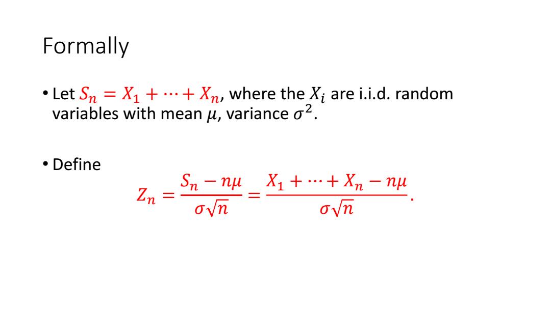
Formally .Let Sm=X1+..+Xn,where the Xi are i.i.d.random variables with mean u,variance o2. 。Define Sn-nW_X1+…+Xn-nw Zn= 0√m
Formally • Let 𝑆𝑛 = 𝑋1 + ⋯ + 𝑋𝑛, where the 𝑋𝑖 are i.i.d. random variables with mean 𝜇, variance 𝜎 2 . • Define 𝑍𝑛 = 𝑆𝑛 − 𝑛𝜇 𝜎 𝑛 = 𝑋1 + ⋯ + 𝑋𝑛 − 𝑛𝜇 𝜎 𝑛
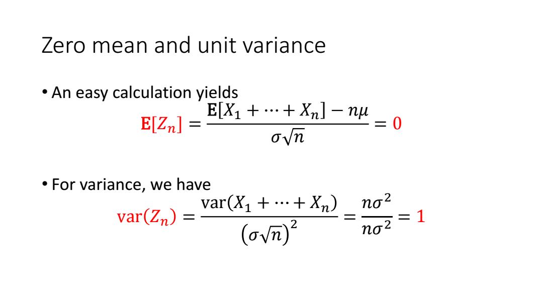
Zero mean and unit variance An easy calculation yields E[X1+…+XnJ-nw E[Zn] 二0 ovn ·For variance,we have var(X1+…+Xn) no2 var(Zn)= (Vm列)
Zero mean and unit variance • An easy calculation yields E[𝑍𝑛] = E 𝑋1 + ⋯ + 𝑋𝑛 − 𝑛𝜇 𝜎 𝑛 = 0 • For variance, we have var 𝑍𝑛 = var 𝑋1 + ⋯ + 𝑋𝑛 𝜎 𝑛 2 = 𝑛𝜎 2 𝑛𝜎 2 = 1
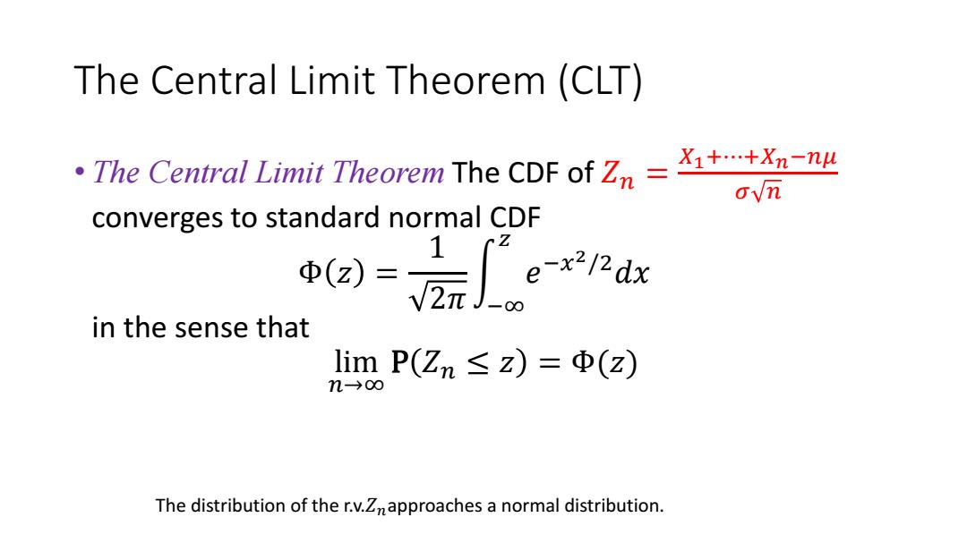
The Central Limit Theorem (CLT) .The Central Limit Theorem The CDF ofZn= X1+.+Xn-nu ovn converges to standard normal CDF in the sense that limP(Zn≤z)=Φ(z) n-→o∞ The distribution of the r.v.Znapproaches a normal distribution
The Central Limit Theorem (CLT) • The Central Limit Theorem The CDF of 𝑍𝑛 = 𝑋1+⋯+𝑋𝑛−𝑛𝜇 𝜎 𝑛 converges to standard normal CDF Φ 𝑧 = 1 2𝜋 න −∞ 𝑧 𝑒 −𝑥 2/2𝑑𝑥 in the sense that lim 𝑛→∞ P 𝑍𝑛 ≤ 𝑧 = Φ(𝑧) The distribution of the r.v.𝑍𝑛approaches a normal distribution
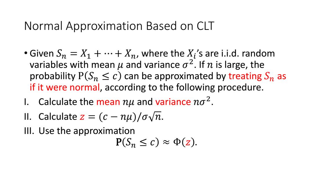
Normal Approximation Based on CLT Given S=X1+.+Xn,where the Xi's are i.i.d.random variables with mean u and variance o2.If n is large,the probability P(Sn<c)can be approximated by treating Sn as if it were normal,according to the following procedure. l. Calculate the mean nu and variance no2. ll.Calculate z (c-nu)/ovn. Ill.Use the approximation P(Sn≤c)≈Φ(z):
Normal Approximation Based on CLT • Given 𝑆𝑛 = 𝑋1 + ⋯ + 𝑋𝑛, where the 𝑋𝑖 ’s are i.i.d. random variables with mean 𝜇 and variance 𝜎 2 . If 𝑛 is large, the probability P 𝑆𝑛 ≤ 𝑐 can be approximated by treating 𝑆𝑛 as if it were normal, according to the following procedure. I. Calculate the mean 𝑛𝜇 and variance 𝑛𝜎2 . II. Calculate 𝑧 = (𝑐 − 𝑛𝜇)/𝜎 𝑛. III. Use the approximation P 𝑆𝑛 ≤ 𝑐 ≈ Φ 𝑧
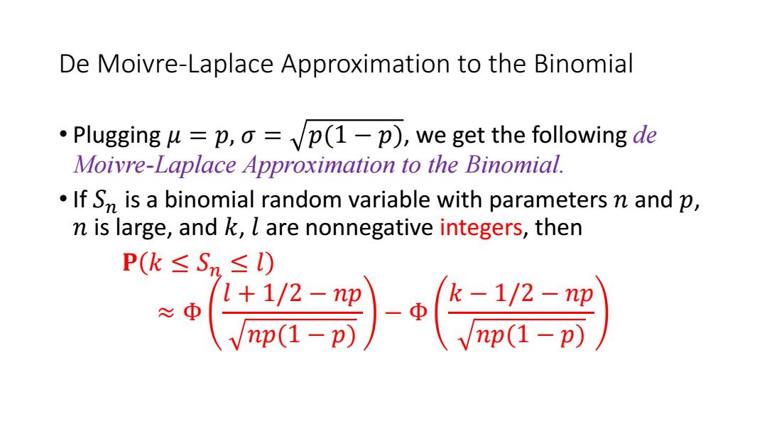
De Moivre-Laplace Approximation to the Binomial Plugging u =p,o =p(1-p),we get the following de Moivre-Laplace Approximation to the Binomial. If Sn is a binomial random variable with parameters n and p, n is large,and k,l are nonnegative integers,then P(k≤Sn≤) 》〉-器》 l+1/2-np ≈中
De Moivre-Laplace Approximation to the Binomial • Plugging 𝜇 = 𝑝, 𝜎 = 𝑝(1 − 𝑝), we get the following de Moivre-Laplace Approximation to the Binomial. • If 𝑆𝑛 is a binomial random variable with parameters 𝑛 and 𝑝, 𝑛 is large, and 𝑘, 𝑙 are nonnegative integers, then 𝐏 𝑘 ≤ 𝑆𝑛 ≤ 𝑙 ≈ Φ 𝑙 + 1/2 − 𝑛𝑝 𝑛𝑝(1 − 𝑝) − Φ 𝑘 − 1/2 − 𝑛𝑝 𝑛𝑝(1 − 𝑝)

Problem 8. Before starting to play the roulette in a casino,you want to look for biases that you can exploit. You therefore watch 100 rounds that result in a number between 1 and 36,and count the number of rounds for which the result is odd. If the count exceeds 55,you decide that the roulette is not fair
Problem 8. • Before starting to play the roulette in a casino, you want to look for biases that you can exploit. • You therefore watch 100 rounds that result in a number between 1 and 36, and count the number of rounds for which the result is odd. • If the count exceeds 55, you decide that the roulette is not fair

Question Assuming that the roulette is fair,find an approximation for the probability that you will make the wrong decision
Question • Assuming that the roulette is fair, find an approximation for the probability that you will make the wrong decision
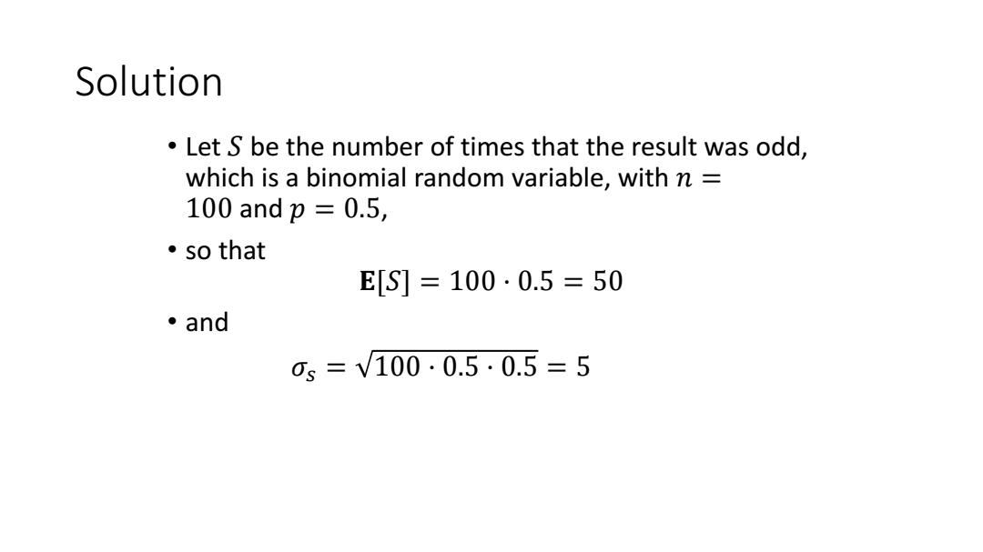
Solution Let s be the number of times that the result was odd, which is a binomial random variable,with n 100andp=0.5, ·so that E[S]=100·0.5=50 。and 0s=V100.0.5·0.5=5
Solution • Let 𝑆 be the number of times that the result was odd, which is a binomial random variable, with 𝑛 = 100 and 𝑝 = 0.5, • so that 𝐄[𝑆] = 100 · 0.5 = 50 • and 𝜎𝑠 = 100 · 0.5 · 0.5 = 5