ENGG2430 ProbabStatistics forners Chapter 3:General Random Variables Instructor: Shengyu Zhang
Instructor: Shengyu Zhang
Content Continuous random variables and PDEs Cumulative Distribution Functions Normal Random Variables Joint PDFs of Multiple Random Variables Conditioning The Continuous Bayes'Rule
Content ◼ Continuous Random Variables and PDFs ◼ Cumulative Distribution Functions ◼ Normal Random Variables ◼ Joint PDFs of Multiple Random Variables ◼ Conditioning ◼ The Continuous Bayes’ Rule

Continuous random variables We've learned discrete random variables. which can be used for dice rolling,coin flipping,etc. Random variables with a continuous range of possible values are quite common. velocity of a vehicle traveling along the highway Continuous random variables are useful: finer-grained than discrete random variables able to exploit powerful tools from calculus
Continuous Random Variables ◼ We’ve learned discrete random variables, which can be used for dice rolling, coin flipping, etc. ◼ Random variables with a continuous range of possible values are quite common. ❑ velocity of a vehicle traveling along the highway ◼ Continuous random variables are useful: ❑ finer-grained than discrete random variables ❑ able to exploit powerful tools from calculus
Continuous r.v.and PDFs A random variable X is called continuous if there is a functionf =0,called the probability density function of X,or PDF,s.t. P(XEB)=fx(x)dx for every subset B R. We assume the integral is well-defined Compared to discrete case:replace summation by integral
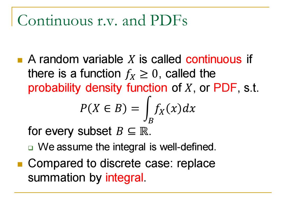
Continuous r.v. and PDFs ◼ A random variable 𝑋 is called continuous if there is a function 𝑓𝑋 ≥ 0, called the probability density function of 𝑋, or PDF, s.t. 𝑃 𝑋 ∈ 𝐵 = න 𝐵 𝑓𝑋 𝑥 𝑑𝑥 for every subset 𝐵 ⊆ ℝ. ❑ We assume the integral is well-defined. ◼ Compared to discrete case: replace summation by integral
PDF In particular,when B [a,b], p(a≤x≤b)=fx()dx is the area under the graph of PDF. PDF fx(x) Sample space b Event {as Xsb}
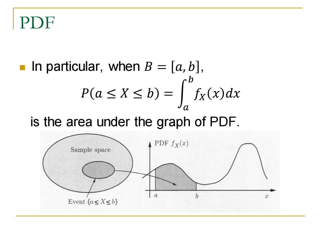
PDF ◼ In particular, when 𝐵 = 𝑎, 𝑏 , 𝑃 𝑎 ≤ 𝑋 ≤ 𝑏 = න 𝑎 𝑏 𝑓𝑋 𝑥 𝑑𝑥 is the area under the graph of PDF
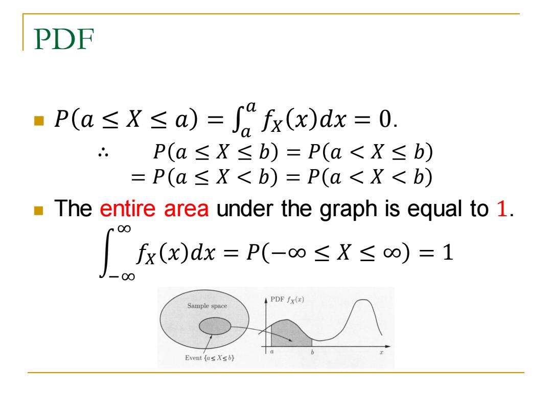
PDF "P(a≤X≤a)=fx(x)dx=0. P(a≤X≤b)=P(a<X≤b) =P(a≤X<b)=P(a<X<b) The entire area under the graph is equal to 1. 00 fx(x)dx=P(-∞≤X≤o)=1 00 PDF fx() Sample space Event (as Xsb}
PDF �� = �� ≥ �� ≥ �� �� ◼ 𝑎 𝑓𝑋 𝑥 𝑑𝑥 = 0. ∴ 𝑃 𝑎 ≤ 𝑋 ≤ 𝑏 = 𝑃 𝑎 < 𝑋 ≤ 𝑏 = 𝑃 𝑎 ≤ 𝑋 < 𝑏 = 𝑃 𝑎 < 𝑋 < 𝑏 ◼ The entire area under the graph is equal to 1. න −∞ ∞ 𝑓𝑋 𝑥 𝑑𝑥 = 𝑃 −∞ ≤ 𝑋 ≤ ∞ = 1
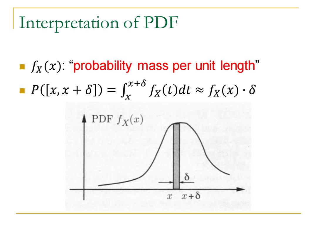
Interpretation of PDF ·fx(x):"“probability mass per unit length'” ■P(x,x+δ)=+fr(t)dt≈fr(o·d PDF fx(x) xE+ò
Interpretation of PDF ◼ 𝑓𝑋(𝑥): “probability mass per unit length” �� = �� + �� ,�� �� ◼ 𝑥+𝛿 𝑓𝑋 𝑡 𝑑𝑡 ≈ 𝑓𝑋(𝑥) ∙ 𝛿
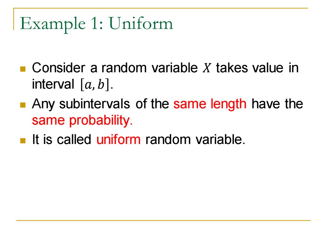
Example 1:Uniform Consider a random variable x takes value in interval [a,b]. Any subintervals of the same length have the same probability It is called uniform random variable
Example 1: Uniform ◼ Consider a random variable 𝑋 takes value in interval 𝑎, 𝑏 . ◼ Any subintervals of the same length have the same probability. ◼ It is called uniform random variable
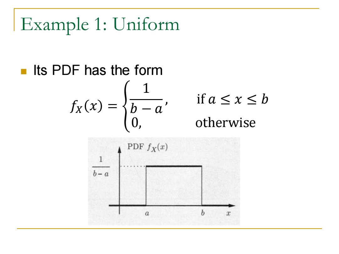
Example 1:Uniform Its PDF has the form 1 0-B-a ifa≤x≤b otherwise PDF fx(z) 1 b-a a b
Example 1: Uniform ◼ Its PDF has the form 𝑓𝑋 𝑥 = ቐ 1 𝑏 − 𝑎 , if 𝑎 ≤ 𝑥 ≤ 𝑏 0, otherwise
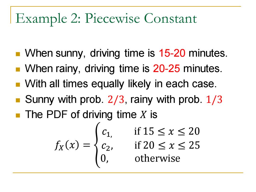
Example 2:Piecewise Constant When sunny,driving time is 15-20 minutes. When rainy,driving time is 20-25 minutes. With all times equally likely in each case. ■ Sunny with prob.2/3,rainy with prob.1/3 The PDF of driving time X is C1, if15≤x≤20 fx(x)= C2, if20≤x≤25 0, otherwise
Example 2: Piecewise Constant ◼ When sunny, driving time is 15-20 minutes. ◼ When rainy, driving time is 20-25 minutes. ◼ With all times equally likely in each case. ◼ Sunny with prob. 2/3, rainy with prob. 1/3 ◼ The PDF of driving time 𝑋 is 𝑓𝑋 𝑥 = ൞ 𝑐1, if 15 ≤ 𝑥 ≤ 20 𝑐2, if 20 ≤ 𝑥 ≤ 25 0, otherwise